This note was first taken when I learnt the machine learning course on Coursera.
Lectures in this week: Lecture 9.

Cost function & Backpropagation

Cost function

Notations

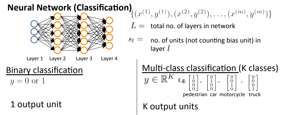
• $L$ = total number of layers in network
• $s_l$ = no. of units (not counting bias unit) in layer $l\in L$

Recall

• Binary classification (review) :
  • $y\in {0,1}$, 1 output unit
  • $h_{\Theta}(x)\in \mathbb{R}$
  • $s_L = 1$ (1 output unit)
  • $K=1$ ($K$ = no. of units in the output layer)
• Multi-class classification with $K$ classes (review): $y\in \mathbb{R}^K$ and K output units
  • $h_{\theta}(x) \in \mathbb{R}^K$
  • $s_L = K$ ($K\ge 3$) because if $K=2$, we can use binary classification.

  

Cost function

• Logistic regression (review here and here):

  $$ J(\theta) = - \frac{1}{m} \displaystyle \sum_{i=1}^m [y^{(i)}\log (h_\theta (x^{(i)})) + (1 - y^{(i)})\log (1 - h_\theta(x^{(i)}))] + \dfrac{\lambda}{2m}\sum_{j=1}^n \theta_j^2. $$

• Neural network (review)

  $$ J(\Theta) = - \frac{1}{m} \sum_{i=1}^m \sum_{k=1}^K \left[y^{(i)}_k \log ((h_\Theta (x^{(i)}))_k) + (1 - y^{(i)}_k)\log (1 - (h_\Theta(x^{(i)}))_k)\right] + \frac{\lambda}{2m}\sum_{l=1}^{L-1} \sum_{i=1}^{s_l} \sum_{j=1}^{s_{l+1}} ( \Theta_{j,i}^{(l)})^2 $$
  • If we want to minimize $J(\Theta)$ as a function of $\Theta$ using one of the advanced optimization methods (fminunc, conjugate gradients, BGGS, L-BFGS, …) we need to supply $J(\Theta)$ and the (partial) gradient derivative terms $\frac{\partial}{\partial \Theta_{ij}^{(l)}}$ for every $i,j,l$.
  • The triple sum simply adds up the squares of all the individual $\Theta$s in the entire network.
  • The $i$ in the triple sum does not refer to training example $i$.

Backpropagation algorithm

Talking about an algorithm to minize the cost function.

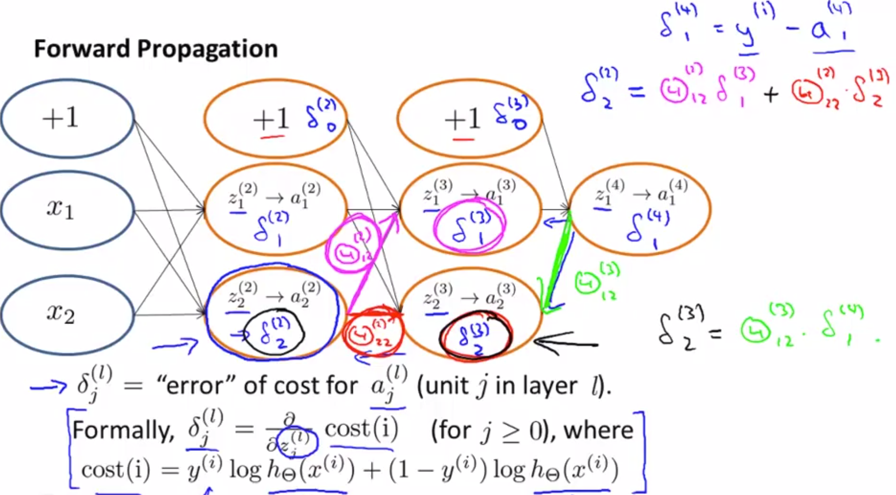
• Forward propagation : from $a^{(1)}$ to the last layer $a^{(L)}$. $\Rightarrow$ computes $h_{\Theta}(x) = a^{(L)} = g(z^{(L)}) = g(\Theta^{(L-1)}a^{(L-1)})$
• Backpropagation : from $a^{(L)}$ back to $a^{(1)}$ $\Rightarrow$ computes the derivative (gradient)

Notations:

• $\delta_j^{(l)}$ = “error” of node $j$ in layer $l$.
• $a_j^{(l)}$ = activation of node $j$ in layer $l$.

For each output unit (layer $L=4$)

or vectorization,

each vecor’s dimension = number of output units.

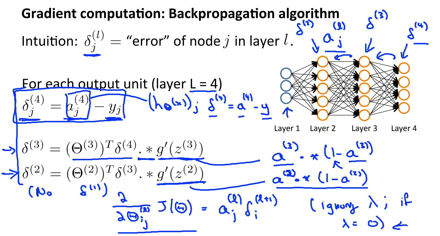
Keep couting $\delta^{(4)}$ to $\delta^{(2)}$. There is no $\delta^{(1)}$ because they are our input dataset, they don’t have any error!

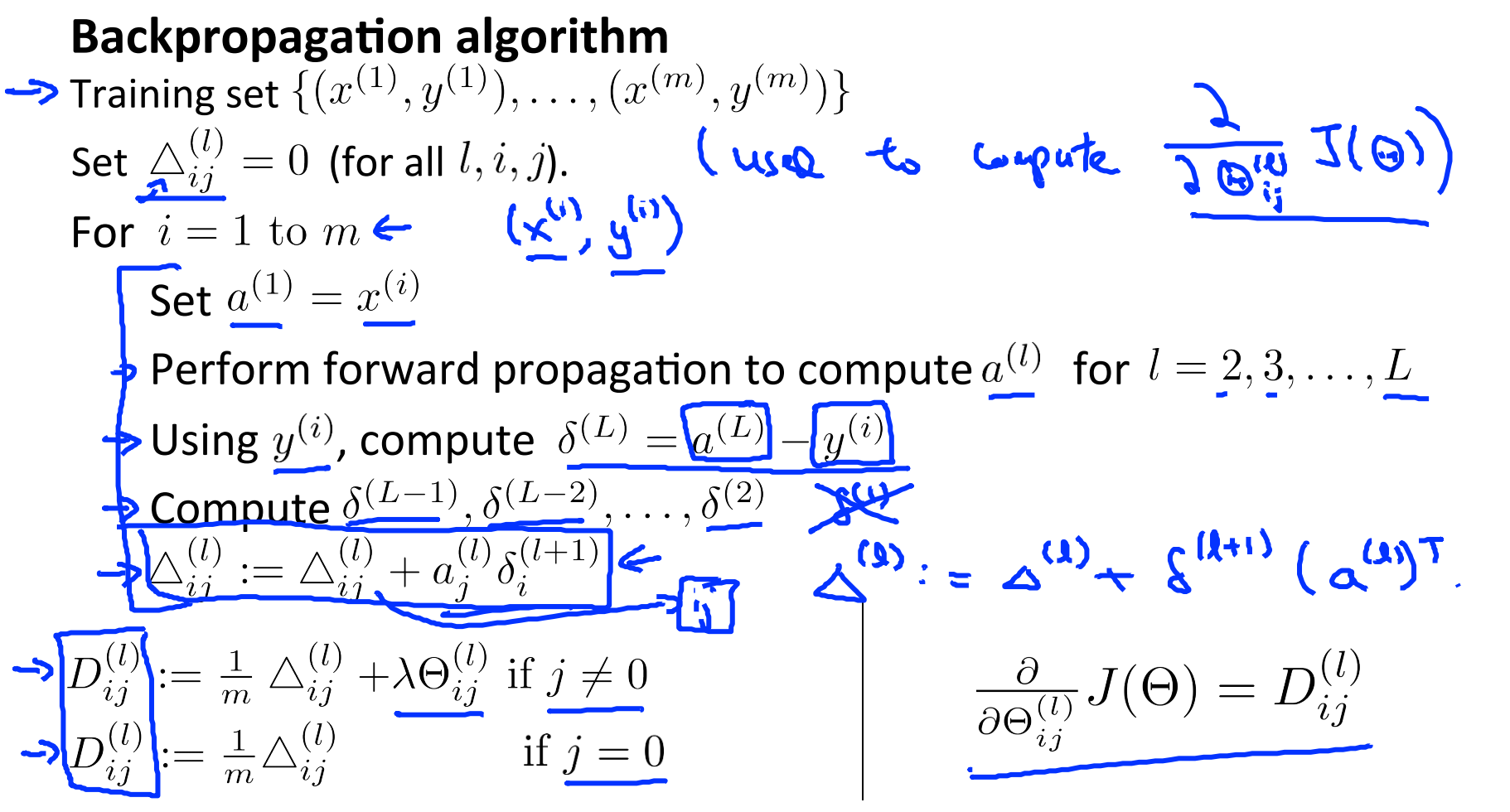
• $\Delta_{ij}^{(l)}$ computes $\frac{\partial}{\partial\Theta_{ij}^{(l)}} J(\Theta)$.

Note that, backpropagation and forward propagation are used alternately inside loop i.

Algorithm

Backpropagation intuition

Backpropagation in practice

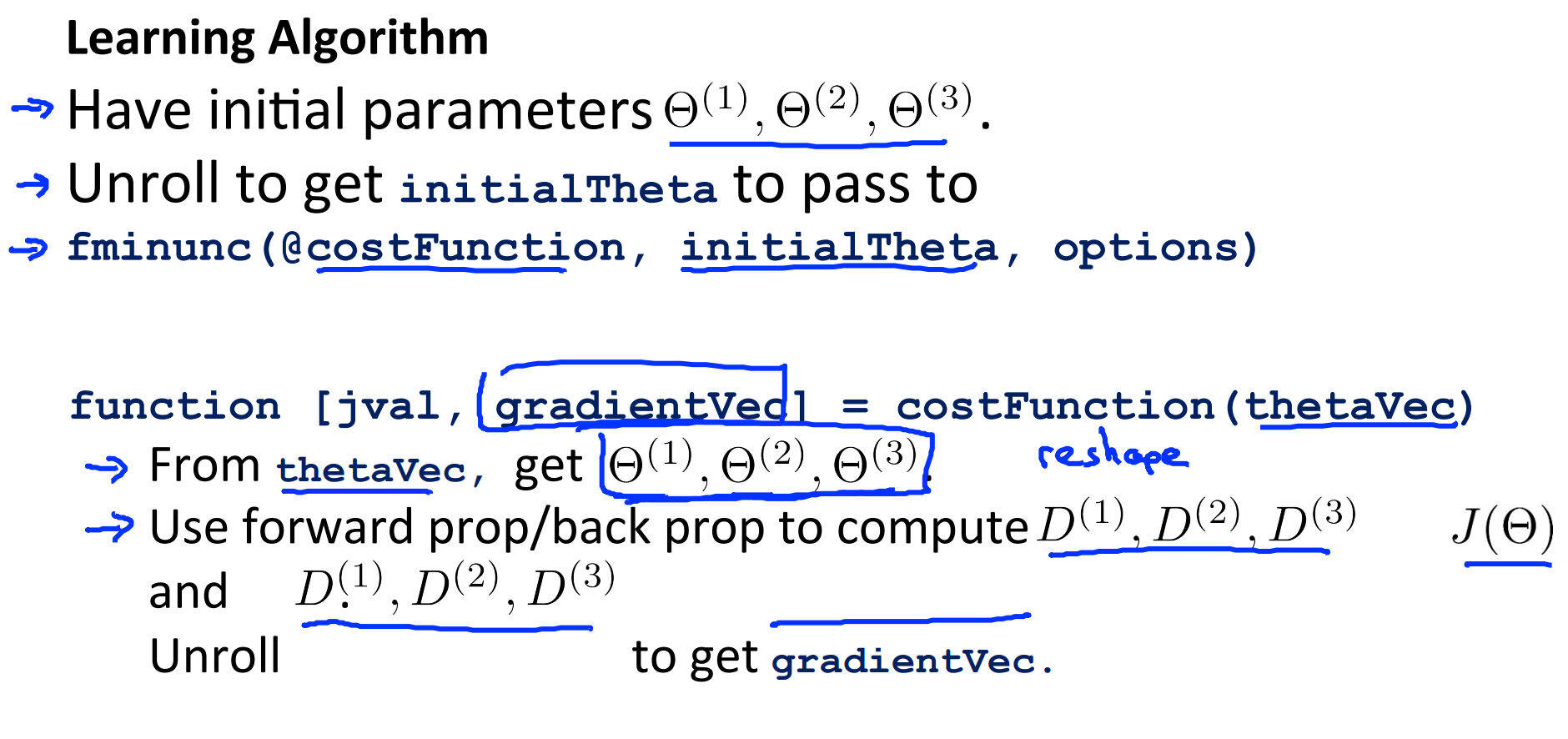
Implementation note: Unrolling parameters

Example:

% make a long vector 
thetaVec = [ Theta1(:); Theta2(:); Theta3(:) ];
DVec = [ D1(:); D2(:); D3(:) ]

If we want to “roll” (get back to each theta),

Theta1 = reshape( thetaVec(1:110), 10, 11 );
Theta2 = reshape( thetaVec(111:220), 10, 11 );
Theta3 = reshape( thetaVec(221:230), 1, 11 );

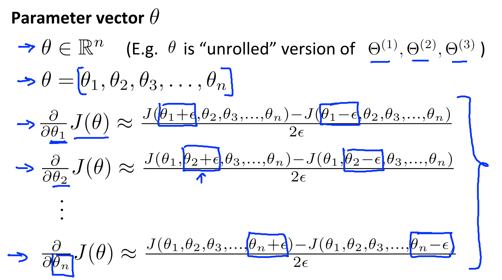
Gradient checking

When implement with backpropagation, there are some subtle error that we don’t know and cannot recognize in which they seems to be right but not. That why we need to always implement gradient checking when working with complex models.

We usually choose $\epsilon = 10^{-4}$.

Implement,

gradApprox = (J(theta + EPSILON) - J(theta - EPSILON)) / (2*EPSILON)

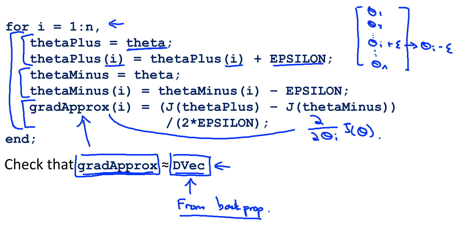
epsilon = 1e-4;
for i = 1:n,
  thetaPlus = theta;
  thetaPlus(i) += epsilon;
  thetaMinus = theta;
  thetaMinus(i) -= epsilon;
  gradApprox(i) = (J(thetaPlus) - J(thetaMinus))/(2*epsilon)
end;

If we have gradApprox $\simeq$ DVec, we can be more confident on the result of DVec and other computations after that.

Practice tips (from exercise)

• When performing gradient checking, it is much more efficient to use a small neural network with a relatively small number of input units and hidden units, thus having a relatively small number of parameters. Each dimension of $\Theta$ requires two evaluations of the cost function and this can be expensive.
• Gradient checking works for any function where you are computing the cost and the gradient. Concretely, you can use the same computeNumericalGradient.m function to check if your gradient implementations for the other exercises are correct too (e.g., logistic regression’s cost function).

Randon initialization

We cannot use initial of $\Theta$ as initialTheta = zeros(n,1) because it will leads to the fact that all $a^{(l)}_j$ are equal too.

We need to initialize $\Theta_{ij}^{(l)}$ to a random values in $[-\epsilon, \epsilon]$, i.e.

Theta1 = rand(10,11) * (2 * INIT_EPSILON) - INIT_EPSILON;
Theta2 = rand(10,11) * (2 * INIT_EPSILON) - INIT_EPSILON;
Theta3 = rand(1,11) * (2 * INIT_EPSILON) - INIT_EPSILON;

When training neural networks, it is important to randomly initialize the parameters for symmetry breaking. One effective strategy for random initialization is to randomly select values for $\Theta^{(l)}$ uniformly in the range $[-\epsilon_{init}, \epsilon_{init}]$.

One effective strategy to choose $\epsilon_{init}$ is to base it on the numbe rof units in the networks. A good choice of $\epsilon\_{init}$ is

where $L_{in} = s_l, L_{out} = s_{l+1}$. $s_l$ is the no. of units (not counting bias unit) in layer $l$.

Putting it together

1. Choose a network architecture: choose the number of hidden layers.
   • No. of input units: dim of features $x^{(i)}$
   • No. of output units: number of classes. Note that, we need to write $y$ is the set of separated unit vectors like $y=[1,0,…,0]^T$ or $y=[0,1,0,…,0]^T$,…
   • No. of hidden units: 1 (defaults). If $>1$, should choose the same number of units for each hidden layer.
   • More hidden units $\Rightarrow$ better but more complicated!
2. Training a neural network:
   1. Random initialize weights : small near zero.
   2. Implement forward propagation to get $h_{\Theta}(x^{(i)})$ from $x^{(i)}$
   3. Implement code to compute cost function $J(\Theta)$

   4. Implement backprop to compute partial derivatives $\frac{\partial}{\partial\Theta_{jk}^{(l)}}J(\Theta)$.

      Need to use foor-loop through all of $(x^{(i)}, y^{(i)})$ for i=1:m. Should do that instead of not using it (Andrew recommend!!!).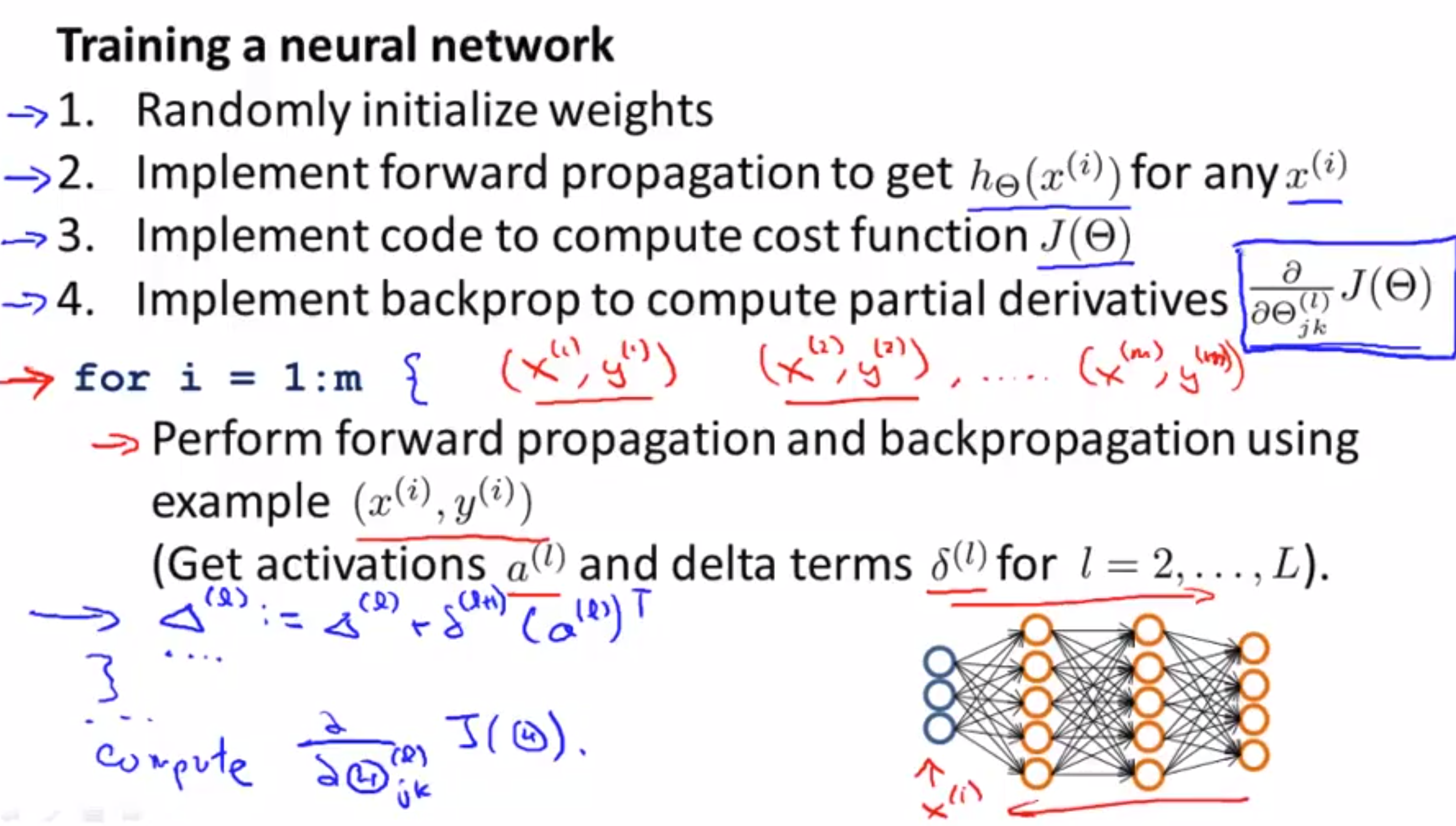

      

   5. Use gradient checking to compare $\frac{\partial}{\partial \Theta_{jk}^{(l)}}J(\Theta)$ computed using backprop vs. using numerical estimate of gradient of $J(\Theta)$. Don’t forget to disable gradient checking code!!!
   6. Use gradient descent or advanced optimization method with backprop to try to minimize $J(\Theta)$ as a function of $\Theta$.

   On neural network, cost function is non convex. Therefore, methods can (theoritically) stuck on local optimal. But in practice, it’s not a huge problem!

Exercise de programmation: Neural network learning

Feedforward and cost function

nnCostFunction.m: Recall that,

A very important remark, in the formulas (without regularization)

$y$ originally is in $\mathbb{R}^{m\times 1}$ but we need to convert it to $y_{new} \in \mathbb{R}^{m\times K}$ like in this section.

$y_k$ is only corresponding to $(h_{\Theta})_k$ for $k$ in output units. We cannot multiply matrix $y$ ($m\times K$) with matrix $h_{\Theta}$ ($m\times K$) because they will multiply all of rows and columns including some components like $y_k$ with $(h_{\Theta})_{k’\ne k}$.

a1 = [ones(m, 1) X]; % add column 1 to a1 (or X), m x 401
z2 = a1 * Theta1'; % m x 25
a2 = sigmoid(z2); % m x 25
a2 = [ones(m, 1) a2]; % add column 1 to a2, m x 26
z3 = a2 * Theta2'; % m x 10
h = sigmoid(z3); % m x 10

ynew = (1:num_labels) == y;
J = (-1/m) * sum(sum( ynew .* log(h) + (1-ynew) .* log(1-h) ));

Regularized cost function

Also in nnCostFunction.m.

• Above formulas is just an example for this specific test, the code should work for any number of layers and units! ($\Theta^{(1)}$, \Theta^{(2)}) for any size.
• Don’t regularize terms corresponding to the bias (first column of Theta1 and Theta2).

J = J + lambda/(2*m) * ( sum(sum(Theta1(:,2:end).^2)) + sum(sum(Theta2(:,2:end).^2)) );

Sigmoid gradient

File sigmoidGradient.m.

g = sigmoid(z) .* (1 - sigmoid(z));

Random initialization

File randInitializeWeights.m.

epsilon_init = 0.12;
W = rand(L_out, 1 + L_in) * 2 * epsilon_init - epsilon_init;

Backpropagation

File nnCostFunction.m again.

• Theta1_grad $\in \mathbb{R}^{25 \times 401}$ (like $\Theta^{(1)}$)
• Theta2_grad $\in \mathbb{R}^{10 \times 26}$ (like $\Theta^{(2)}$)

However, when we apply ($\Delta^{(1)}$ is corresponding to Theta1_grad and the same for 2)

with $\delta^{(2)} \in \mathbb{R}^{1\times 26}, a^{(1)} \in \mathbb{R}^{1\times 401}$, the result we obtain is $\Delta^{(1)} \in \mathbb{R}^{26\times 401}$ not $25 \times 401$. That’s why we need to remove/ignore $\delta^{(2)}_0$. For $\delta^{(3)} \in \mathbb{R}^{1\times 10}, a^{(2)}\in \mathbb{R}^{1\times 26}$, we don’t need to do that because the dimension is satisfied.

Note that, loop through all examples (1:m), that’s why we have $\Delta^{(1)} = \Delta^{(1)} + …$.

% in section Part 2

D1 = zeros(size(Theta1)); % 25 x 401
D2 = zeros(size(Theta2)); % 10 x 26
for t=1:m
    % step 1
    a1 = [1, X(t, :)]; % 1 x 401
    z2 = a1 * Theta1'; % 1 x 25
    a2 = [1, sigmoid(z2)]; % 1 x 26
    z3 = a2 * Theta2'; % 1 x 10
    a3 = sigmoid(z3); % 1 x 10
    
    % step 2
    sig3 = a3 - ynew(t,:); % 1 x 10
    
    % step 3
    sig2 = (sig3 * Theta2) .* a2 .* (1-a2); % 1 x 26
    
    % step 4
    D1 = D1 + transpose(sig2(2:end)) * a1; % 25 x 401
    D2 = D2 + sig3' * a2; % 20 x 26
end
Theta1_grad = 1/m * D1;
Theta2_grad = 1/m * D2;

Gradient checking

File computeNumericalGradient.m.

numgrad = zeros(size(theta));
perturb = zeros(size(theta));
e = 1e-4;
for p = 1:numel(theta)
    % Set perturbation vector
    perturb(p) = e;
    loss1 = J(theta - perturb);
    loss2 = J(theta + perturb);
    % Compute Numerical Gradient
    numgrad(p) = (loss2 - loss1) / (2*e);
    perturb(p) = 0;
end

Regularized Neural Networks

Theta1_grad(:,2:end) = Theta1_grad(:,2:end) + lambda/m * Theta1(:,2:end);
Theta2_grad(:,2:end) = Theta2_grad(:,2:end) + lambda/m * Theta2(:,2:end);