
ML Coursera 3 - w3: Logistic Regression
Posted on 11/09/2018, in Machine Learning.This note was first taken when I learnt the machine learning course on Coursera.
Lectures in this week: Lecture 6, Lecture 7.
Classification & Representation
Classification
-
Variable $y$ has discrete values.
-
Other name of : 1 (positive class), 0 (negative class) $\Rightarrow$ binary classification problem
-
If y has more than 2 values, it’s called multi classification
-
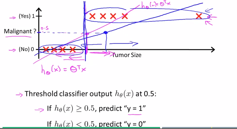
Using linear regression in this case seems not to be very good because there may be some values that effects much more than the others (blue line).
-
$h_{\theta}$ may take values >1 or <0 but we want $0\le h_{\theta} \le 1$. That’s why we need logistic regression, i.e. $h_{\theta}$ is always between $[0,1]$
-
Remember and not confused that logistic regression is just a classification regression in cases of y taking discrete values.
Hypothesis representation
-
What is the function we are going to use to represent the hypothesis
-
Logistic regression
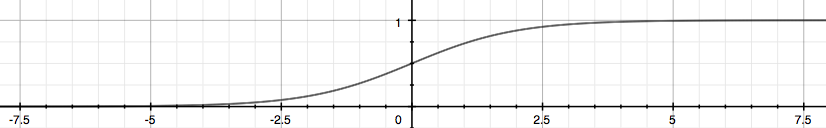
- They are the same: sigmoid function = logistic function = $g(z)$
-
Some propabilities
$$ \begin{align*}& h_\theta(x) = P(y=1 | x ; \theta) = 1 - P(y=0 | x ; \theta) \newline& P(y = 0 | x;\theta) + P(y = 1 | x ; \theta) = 1\end{align*} $$
Decision Boundary
From the above figure, we see that
We have
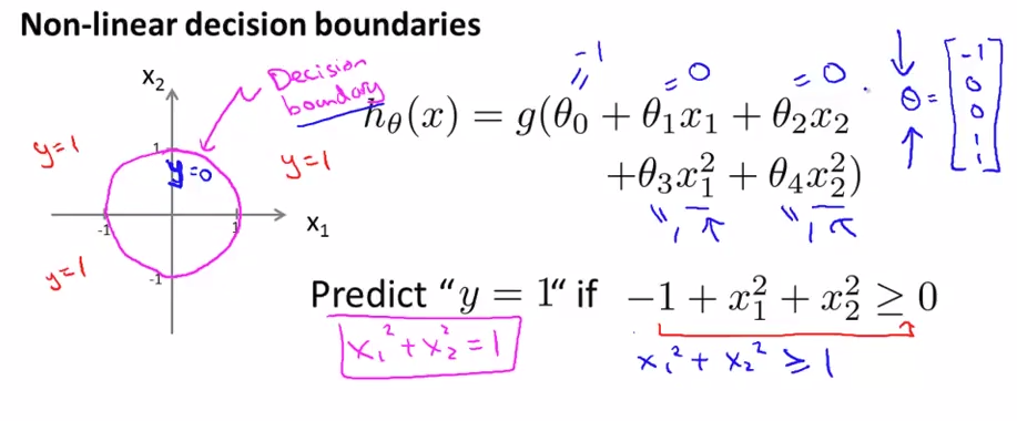
The decision boundary is the line that separates the area where y = 0 and where y = 1mark>. It is created by our hypothesis function.
An example,
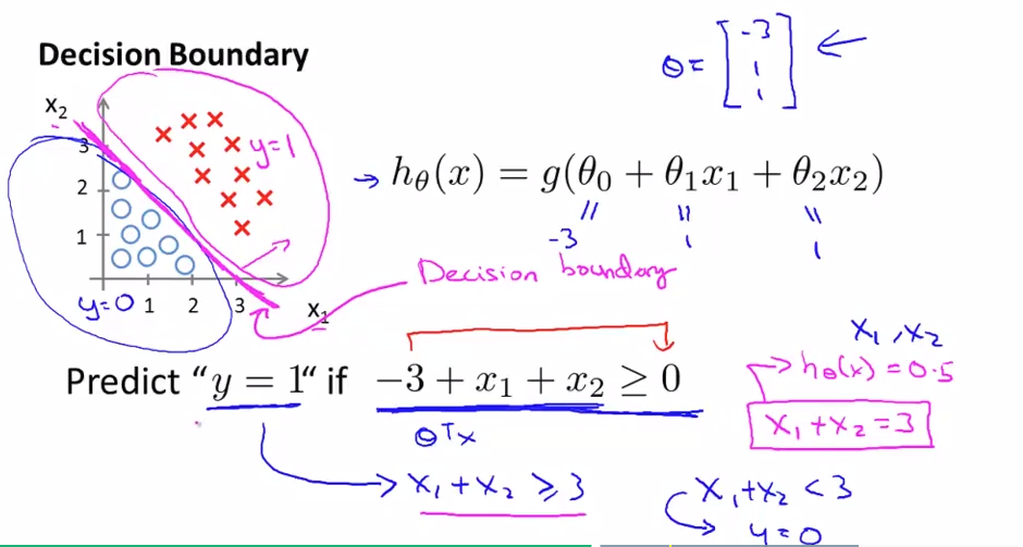
The training set is not used to determine the decision boundary, but parameter $\theta$. The training set is used only for fit the parameter $\theta$.
Logistic regression model
Cost function
or we can write,
The cost function is rewritten as
Vectorization
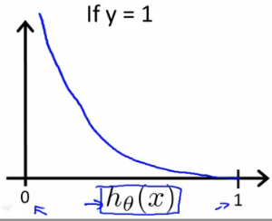
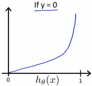
- If hypothesis seems to be “wrong” ($h \to 1$ while $y\to 0$ or $h \to 0$ while $y\to 1$) then $\text{Cost}\to \infty$
- $J(\theta)$ ins this style is always convex.
Simplified Cost Function and Gradient Descent
In this logistic regression,
Notice that, above equation looks the same with one in linear regression, the different is def of $h_{\theta}$!
Vectorization
Advanced Optimization
“Conjugate gradient”, “BFGS”, and “L-BFGS” are more sophisticated, faster ways to optimize $\theta$ that can be used instead of gradient descent. We suggest that you should not write these more sophisticated algorithms yourself (unless you are an expert in numerical computing) but use the libraries instead, as they’re already tested and highly optimized. Octave/Matlab provides them.
A single function that returns both $J(\theta)$ and $\frac{\partial}{\partial\theta_j}J(\theta)$
function [jVal, gradient] = costFunction(theta)
  jVal = [...code to compute J(theta)...];
  gradient = [...code to compute derivative of J(theta)...];
end
Then we can use octave’s fminunc() optimization algorithm along with the optimset() function that creates an object containing the options we want to send to fminunc().
options = optimset('GradObj', 'on', 'MaxIter', 100);
initialTheta = zeros(2,1);
[optTheta, functionVal, exitFlag] = fminunc(@costFunction, initialTheta, options);
We give to the function fminunc() our cost function, our initial vector of theta values, and the options object that we created beforehand.
info
fmincg works similarly to fminunc, but is more more efficient for dealing with a large number of parameters.
Multiclass classification: one-vs-all
$y$ has more values than only two 0 and 1. We keep using binary classification for each group of 2 (consider one and see the others as the other group)
(n+1)-values $y \Rightarrow n+1$ binary classification problems.
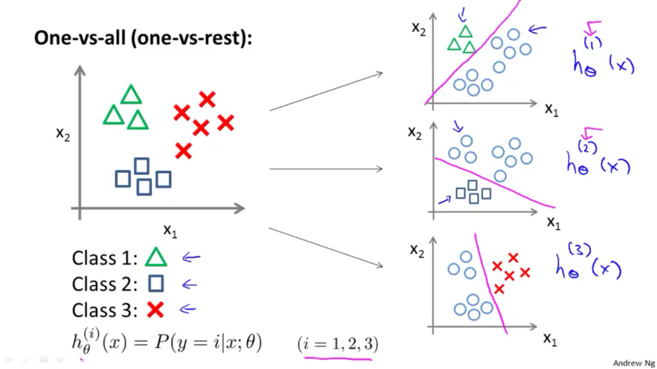
After fiding optTheta from fmincg, we need to find $h_{\theta}$. From $h_{\theta}$ for all classes, we find the one with the highest propability (highest $h$). That’s why we have the line of code prediction above.
-
face Why max?
We want to choose a $\Theta$ such that for all $j\in \{ 0,\ldots,n \}$,
Don’t forget that, we consider $h_{\theta} \ge 0.5$ as true. Because of that, there is onlty 1 option, that’s max of all $j$.
info See ex 4 for an example in practice.
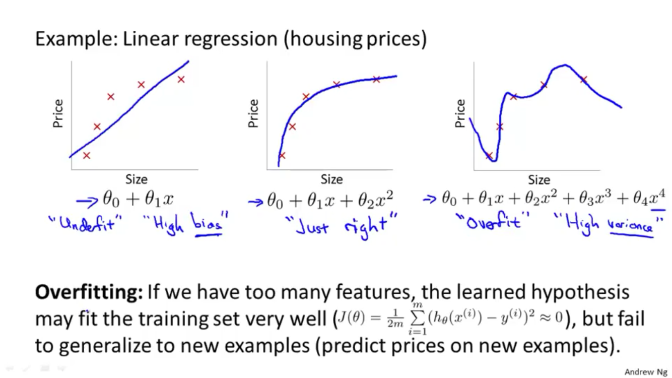
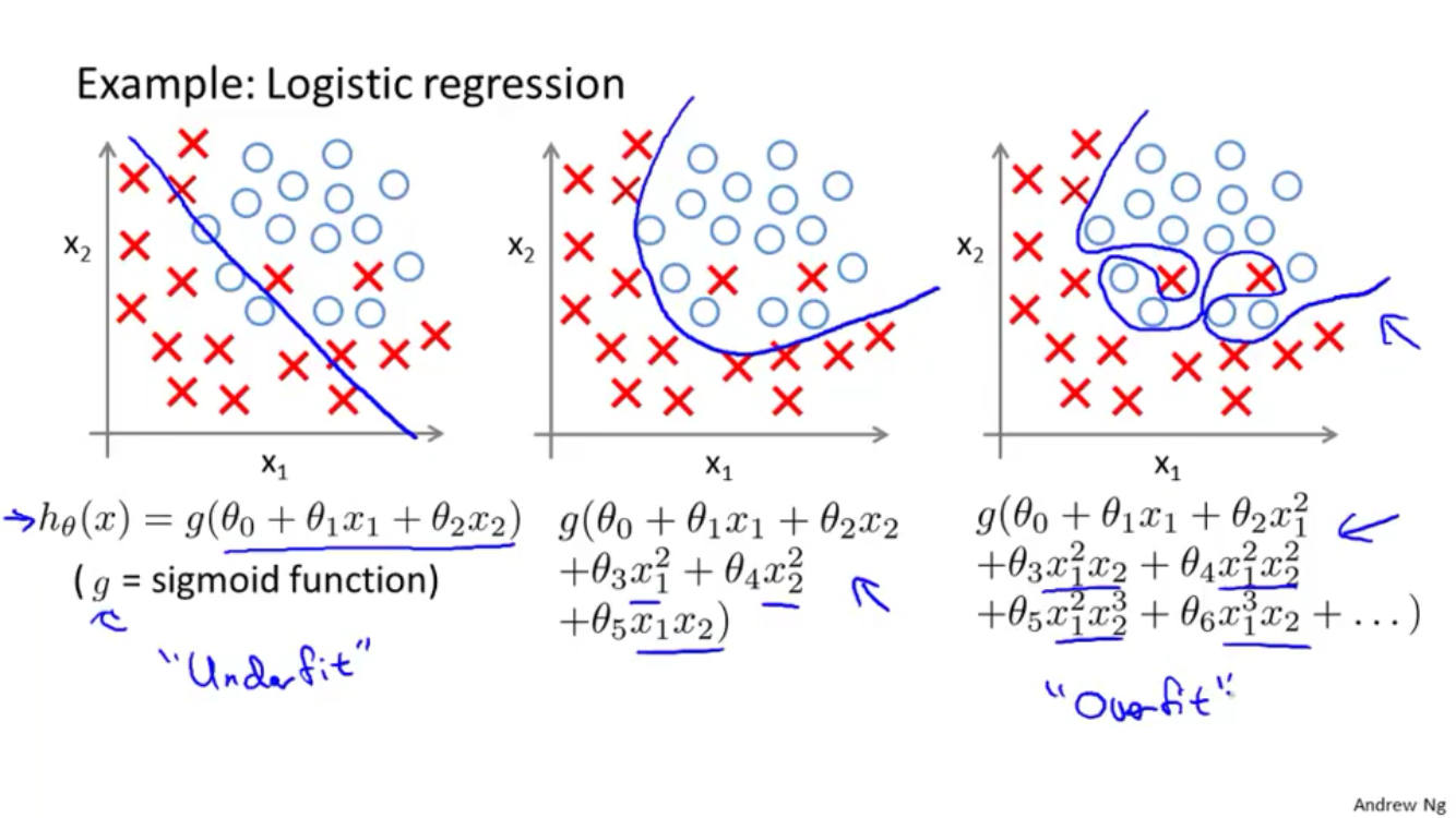
Solving the problem of overfitting
The problem of overfitting
We have many features, $h_{\theta}$ may fit the training set very well ($J(\theta) \simeq 0$) but fail to generalize.
Cost function
Options to solve:
- Reduce the number of features
- Manually select which features to keep
- By algorithm
- Regularization (add penalty terms)
- Keep all features but reduce magnitude/values of parameters $\theta_j$
- Works well when we have a lot of features, each of which contributes a bit to predicting $y$
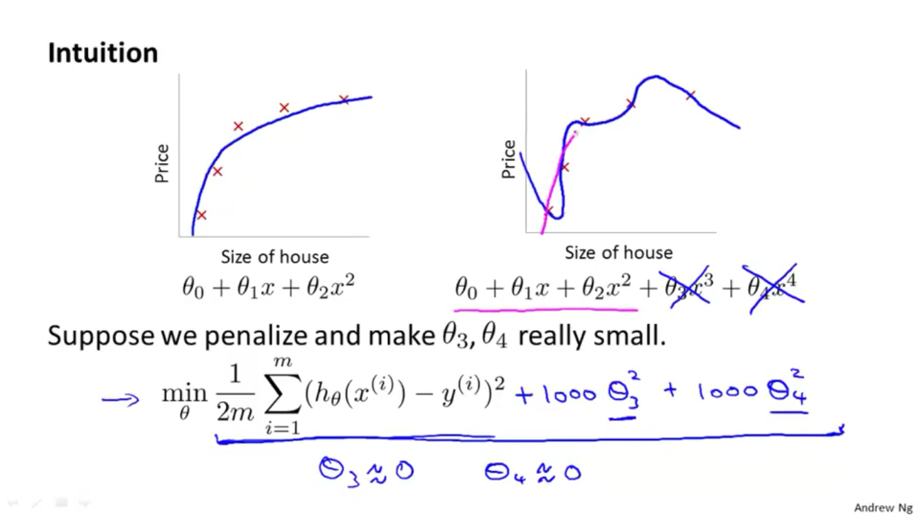
Because we need to find the minimum, we multiply $\theta_3, \theta_4$ by 1000 to make them very big and never be a min, i.e. they look like 0.
If $\lambda$ is too large, the problem of underfitting occurs!
Regularized linear regression
Gradient Descent
Repeat{
}
Intuitively, reduce $\theta_j$ by some amount on every update, the second term is exactly the same it was before.
Normal equation
- $X$ : $m\times (n+1)$ matrix
- $m$ training examples, $n$ features.
- We don’t include $x_0$.
- If $m<n$ then $X^TX$ is non-invertible, but after adding $\lambda\cdot L$, $X^TX + \lambda\cdot L$ becomes invertible!
Regularized logistic regression
We can regularize this equation by adding a term to the end:
And the gradient descent
Repeat{
}
The same form with GD regularized linear regression, the difference in this case is only the definition of $h_{\theta}(x)$
Exercice de programmation: Logistic Regression
Logistic Regression
-
plotData: Plot from
X,yto separate two kind ofXXPos = X(y==1, :); XNeg = X(y==0, :); plot(XPos(:,1), XPos(:,2), 'k+', 'LineWidth', 2, 'MarkerSize', 7); plot(XNeg(:,1), XNeg(:,2), 'ko', 'MarkerFaceColor', 'y', 'MarkerSize', 7); -
sigmoid.m: recall that
g = 1 ./ (1 + exp(-z)); -
costFunction.m: recall that, the cost function in logistic regression is
or in vectorization,
and its gradient is
or in vectorization,
$$ \nabla \theta = \dfrac{1}{m} X^T(g(X\theta) - y). $$h = sigmoid(X*theta); % hypothesis J = 1/m * ( -y' * log(h) - (1-y)' * log(1-h) ); grad = 1/m * X' * ( h - y); fminunc:-
GradObjoption toon, which tells fminunc that our function returns both the cost and the gradientoptions = optimset('GradObj', 'on', 'MaxIter', 400); -
Notice that by using
fminunc, you did not have to write any loops yourself, or set a learning rate like you did for gradient descent.
-
-
predict.m: remember that,
h = sigmoid(X*theta); % m x 1
p = (h >= 0.5);
Regularized logistic regression
costFunctionReg.m: recall that,
its gradient,
h = sigmoid(X*theta); % hypothesis
J = 1/m * ( -y' * log(h) - (1-y)' * log(1-h) ) + lambda/(2*m) * sum(theta(2:end).^2);

grad(1,1) = 1/m * X(:,1)' * (h-y);
grad(2:end,1) = 1/m * X(:,2:end)' * (h-y) + lambda/m * theta(2:end,1);