
ML Coursera 6 - w6: Advice for Applying ML
Posted on 11/10/2018, in Machine Learning.This note was first taken when I learnt the machine learning course on Coursera.
Lectures in this week: Lecture 10, Lecture 11.
Evaluating a Learning Algorithm
Deciding what to try next
Suppose that we have already apply some algorithm of regression but prediction error is bad.
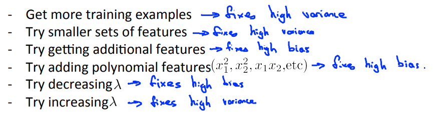
- Get more training examples (more $m$)
- Try smaller sets of features (less $x_i)$
- Try getting additional features (more $x_i)$
- Try adding polynomial features ($x_1^2, x_2^2, x_1x_2,\ldots$)
- Try decreasing or increasing $\lambda$
Evaluating a hypothesis
- If small number of features, we can evaluate easily with a plot to check that a hypothesis is overfitting or not. Bigger number of features may be hard to do in that way.
- Split data into: 70% training cases ($m$) + 30% test cases ($m_{\text{test}}$).
- The new procedure using these two sets is then:
- Learn $\Theta$ and minimize $J_{train}(\Theta)$ using training set.
- Compute the test set error $J_{test}(\Theta)$.
- Misclassification error (0/1 Misclassification error)
Model selection and train/validation/test sets
-
Overfitting example: error measured on training data ($J_{train}$) is likely smaller than the actual generation error.
-
Try with many degree $d$ of polynomial $h$, we can choose the best $d$ based on the error result.
-
An option:
- Training set: 60%
- Cross validation set: 20%
- Test set: 20%
-
Training error
-
Cross validation error
-
Test error
-
Algorithm
- Optimize the parameters in $\Theta$ using the training set for each polynomial degree.
- Find the polynomial degree d with the least error using the cross validation set.
- Estimate the generalization error using the test set with $J_{test}(\Theta^{(d)})$, ($d$ = theta from polynomial with lower error);
Bias vs Variance
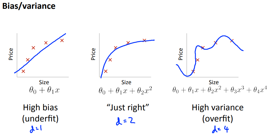
Diagnosing bias vs Variance
- Bad prediction: bias or variance?
- Training error decreases if we increase degree $d$ of the polynomial
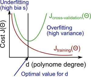
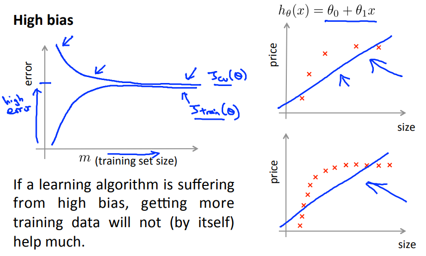
- High bias (underfitting): $J_{train}, J_{cv}$ high and $J_{cv} \simeq J_{train}$.
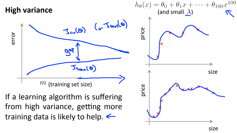
- High variance (overfitting: $J_{train}$ low and $J_{cv} » J_{train}$.
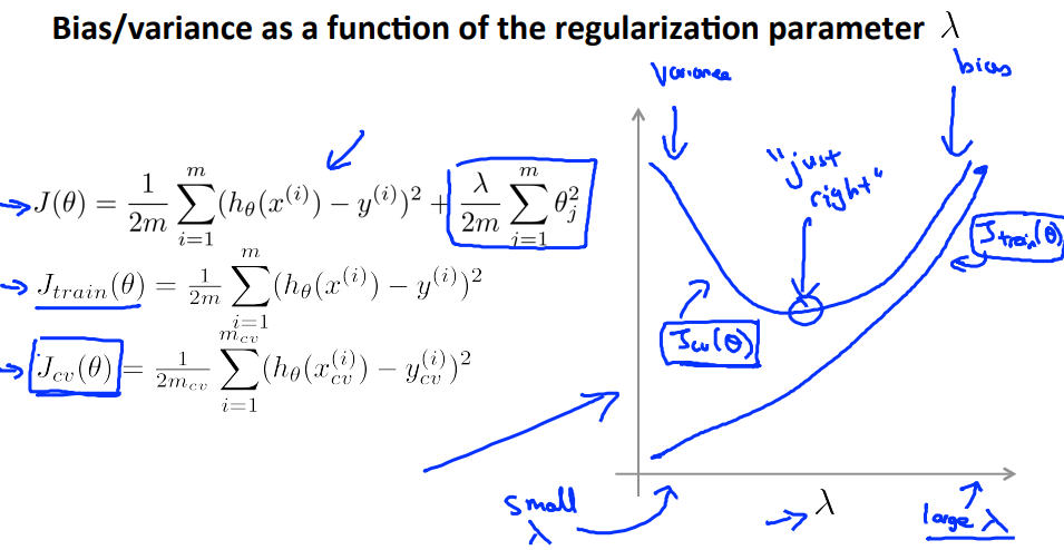
Regularization and Bias/Variance
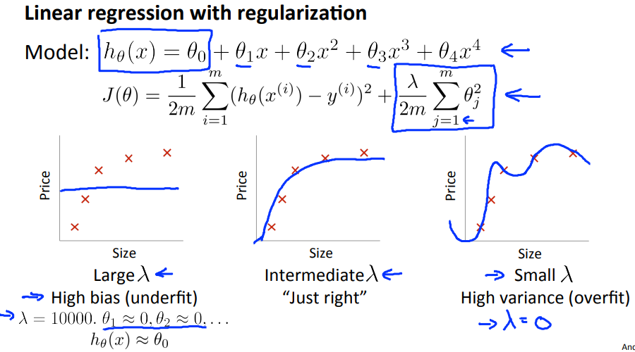
In order to choose the model and the regularization term $\lambda$, we need to:
- Create a list of lambdas (i.e. $\lambda \in \{ 0,0.01,0.02,0.04,0.08,0.16,0.32,0.64,1.28,2.56,5.12,10.24 \}$);
- Create a set of models with different degrees or any other variants.
- Iterate through the $\lambda$s and for each \lambdaλ go through all the models to learn some $\Theta$.
- Compute the cross validation error using the learned $\Theta$ (computed with $\lambda$) on the $J_{CV}(\Theta)$ without regularization or $\lambda = 0$.
- Select the best combo that produces the lowest error on the cross validation set.
- Using the best combo $\Theta$ and $\lambda$, apply it on $J_{test}(\Theta)$ to see if it has a good generalization of the problem.
Learning Curves
- Learning curve plots training and cross validation error as a function of training set size.
- If we add more training examples, it doesn't mean we will get a better result because it also depends on the degree of polynomial we choose (high bias - underfitting).
- In the case of high variance (overfitting). increase the number of training examples seem helps.
Deciding what to do next (revisited)
Exercise the programmation
Regularized Linear Regression
Note that, in the previous notes, there is no vectorized form of this regression. I will list it in this section.
-
Normal form,
-
Vectorized form,
$$ J(\Theta) = \dfrac{1}{2m} (X\Theta - y)^T(X\Theta - y) + \dfrac{\lambda}{2m}\Theta(1:n)^T\Theta(1:n) $$ -
Its gradient,
-
Vetorized form,
$$ \begin{align} \nabla\Theta(0) &= \dfrac{1}{m} X^T(X\Theta - y), \\ \nabla\Theta(1:n) &= \dfrac{1}{m} X^T(X\Theta - y) + \dfrac{\lambda}{2m}\Theta(1:n). \end{align} $$
File linearRegCostFunction.m,
h = X * theta; % hypothesis
J = 1/(2*m) * (X*theta - y)' * (X*theta - y)...
        + lambda/(2*m) * sum(theta(2:end).^2);

grad(1,1) = 1/m * X(:,1)' * (h-y);
grad(2:end,1) = 1/m * X(:,2:end)' * (h-y) + lambda/m * theta(2:end,1);
Because our current implementation of linear regression is trying to fit a 2-dimensional $\Theta$, regularization will not be incredibly helpful for a $\Theta$ of such low dimension.
Bias variance
File learningCurve.m. Note that, we want to validate the quality of $\Theta$ obtained from the training set, that why we use the same theta for both error_train and error_val. We should compute cross validation error on the entire Xval, yval set instead of a part like train set.
for i = 1:m
    theta = trainLinearReg(X(1:i,:), y(1:i), lambda);
    [error_train(i), ~] = linearRegCostFunction(X(1:i,:), y(1:i), theta, 0);

    [error_val(i), ~] = linearRegCostFunction(Xval, yval, theta, 0);
end
Polynomial regression
File polyFeatures.m. The problem with our linear model was that it was too simple for the data and resulted in underfitting (high bias). In this part of the exercise, you will address this problem by adding more features.
for i=1:p
   X_poly(:,i) = X(:,1).^i;
end
Selecting $\lambda$ using a cross validation set
In particular, a model without regularization ($\lambda = 0$) fits the training set well, but does not generalize. Conversely, a model with too much regularization ($\lambda=100$) does not fit the training set and testing set well. A good choice of $\lambda$ (e.g., $\lambda=1$) can provide a good fit to the data.
File validationCurve.m. In this section, you will implement an automated method to select the $\lambda$ parameter. Concretely, you will use a cross validation set to evaluate how good each $\lambda$ value is. After selecting the best $\lambda$ value using the cross validation set, we can then evaluate the model on the test set to estimate how well the model will perform on actual unseen data.
for i = 1:length(lambda_vec)
    lambda = lambda_vec(i);
    theta = trainLinearReg(X, y, lambda);
    [error_train(i), ~] = linearRegCostFunction(X, y, theta, 0);
    [error_val(i), ~] = linearRegCostFunction(Xval, yval, theta, 0);
end
Building A spam classifier
We talk about Machine Learning system design.
Prioritizing what to work on
So how could you spend your time to improve the accuracy of this classifier?
- Collect lots of data (for example “honeypot” project but doesn’t always work)
- Develop sophisticated features (for example: using email header data in spam emails)
- Develop algorithms to process your input in different ways (recognizing misspellings in spam).
- It is difficult to tell which of the options will be most helpful.
Error analysis
Recommended approach
- Start with simple algorithm that you can implement quickly. Implement it and test it on your cross-validation data
- Plot learning curves to decide if more data, more features,… are likely to help.
- Manually examine the errors on examples in the cross validation set and try to spot a trend where most of the errors were made.
- It is very important to get error results as a single, numerical value. Otherwise it is difficult to assess your algorithm’s performance.
- Most of the time the simplest method is the most correct one.
- So once again, take a quick and dirty way to implement the algorithms. From the result , we will then spend some time wisely go which the direction of complexity of the learning algorithm for particular set of problems.
Handling skewed data
Error metrics for skewed classes:
Skewed classes: a somewhat trickier problem to handle with error analysis.
- This is cancer examples, where we have 1% error test. Suppose to be good learning algorithm?
- But as it turns out, the cancer patients only 0.50%. If we set the function that ignore X, only set y = 0 all the time(set all patients don’t have cancer), then automatically we have 0.5% error test. EVEN BETTER!(sarcastically)
- If this the problem, then it is called Skewed classes. And become much harder problem. Skewed classes: The data that we have turns out not balance, it weight more to one class than the other
- Which turns out ignore the data is more correct than incorporating data.
- The solution? Even improving the accuracy of the algorithms, it still lack the prediction of real overall output
-
Better come up with different metrics
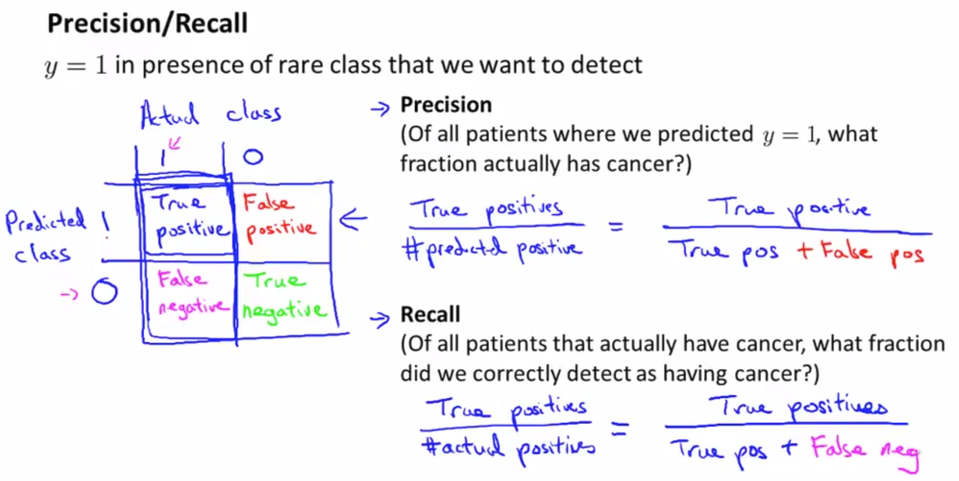
- Precision : the ratio of patients actually have cancer based on all cancer prediction (actual positive/predicted positive)
- Recall: the ratio of correctly tell them if they are indeed have a cancer. The higher the recall, the better our learning algorithm.
- Using these, in skew classes, there’s no possible to cheat ( 0 or 1 all the time). For example if we set y = 0(all patients don’t have cancer) all the time, then we would have recall = 0. That is we can’t predict at all whether or not the patients have cancer.
- With Precision/Recall , we can tell how’s the algorithm is doing well even if we have skew classes. Good error metrics for evaluation classifier for skewed classes rather than just classification error/accuracy.
Trading off precision and recall
We don’t want to take $h_{\Theta}\ge 0.5$ as before in some cases because of there may be a low recall (i.e. we predict someone that doesn’t have cancer bue they do). Instead of $0.5$, we need to choose another threshold, but how many?
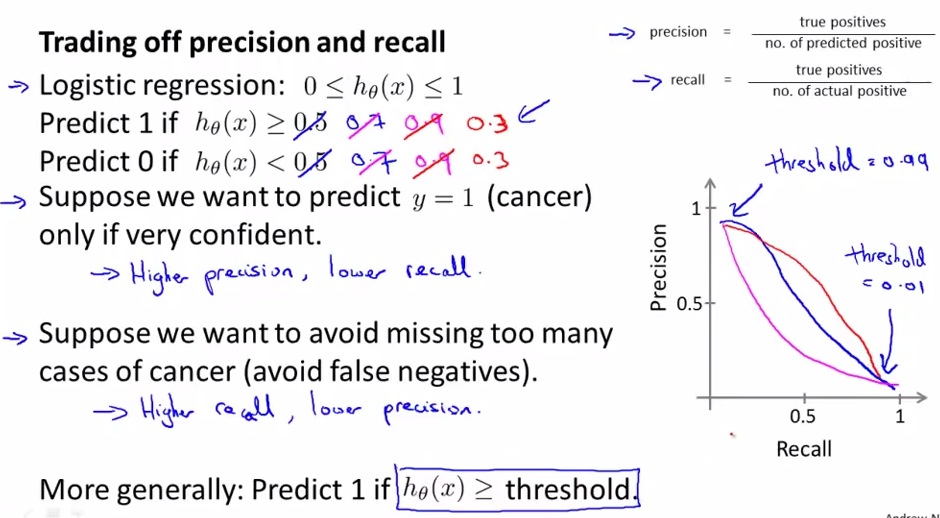
- The intermediate value between 0 and 1 still give a reasonable value.
- If we increase threshold, precision increases but recall decreases.
- Threshold offers a way to control trade-off between precision and recall
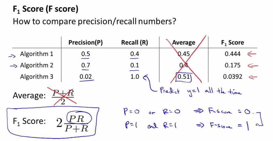
- Fscore gives a single real number evaluation metric (if we use both precision and recall, it’s harder to choose because there are 2 numbers for evaluating)
- If you’re trying to automatically set the threshold, one way is to try a range of threshold values and evaluate them on your cross validation set
- Then pick the threshold which gives the best fscore.
Using large data sets
Data for machine learning
How much data quotient to train on?
- Take an algorithm, give it more data, should beat a “better” one with less data. Shows that
- Algorithm choice is pretty similar
- More data helps????
- When is this true and when is it not?
- If we can correctly assume that features x have enough information to predict y accurately, then more data will probably help
- Another way to think about this is we want our algorithm to have low bias and low variance
- Low bias –> use complex algorithm
- Low variance –> use large training set