This note was first taken when I learnt the machine learning course on Coursera.
Lectures in this week: Lecture 13, Lecture 14.

error This note of Alex Holehouse is also very useful (need to be used alongside with my note).

Clustering

Unsupervised Learning

• This is the first unsupervised learnig.
• There is no label associated to it.
• There is X but not y.
• Unsupervised learning
  • Try and determining structure in the data
  • Clustering algorithm groups data together based on data features

K-means Algorithm

• The most popular and widely used algorithm.
• See here for the figure of idea

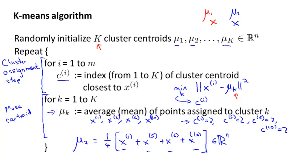
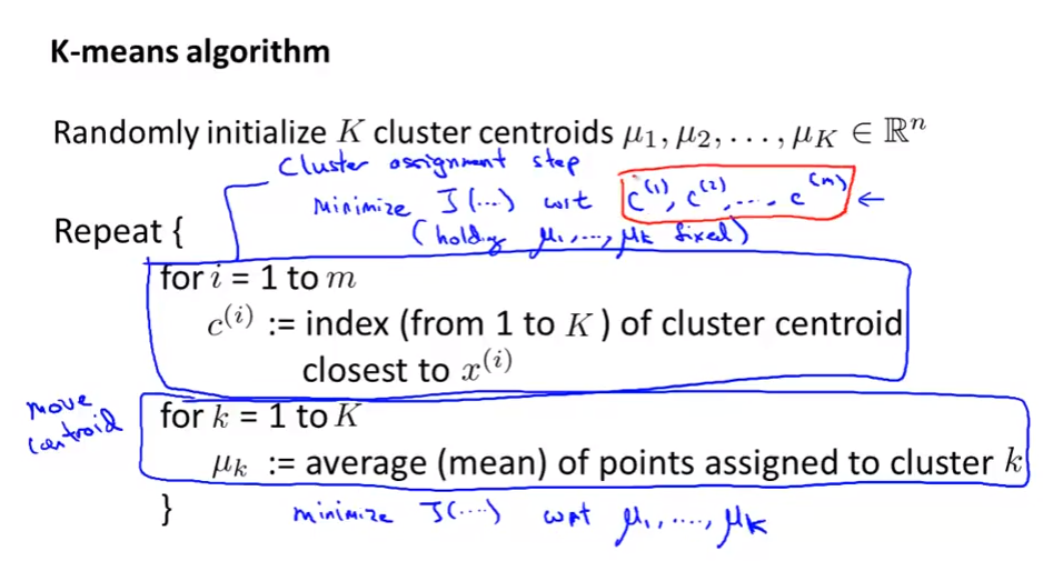
• Algorithm: Cluster assignment step and Move centroid step

  

Optimization objective

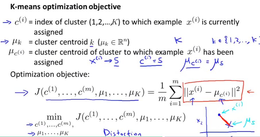
• K-means also have an optimization objective (cost function like supervised learning)
• Knowing this is helpful because
  • Help for debugging
  • Help find better clustering

• distortion cost function

  

• Minimize to find out the $c^{(i)}$ and $\mu_{c^{(i)}}$

  

Random Initialization

• Also talk about how to avoid local optimal as well.
• $K$: number of clusters, $m$: the number of training examples (usually $K<m$)
• Random choose $K$ training examples as a initial cluster.
  • If we choose the wrong examples, it may lead to a local optima
  • To avoid that, dun random K-means multiple times (100 times, for example)
    • Give 100 diff ways to K
    • Choose the one make $J$ min
    • Only apply when $K=2,...,10$

Choosing the number of clusters

• Elbow method: check the cost function J wrt number of clusters.
  • Check the “elbow” (cái cùi chỏ) where the graph change direction much.
  • EM isn't used very often!

  

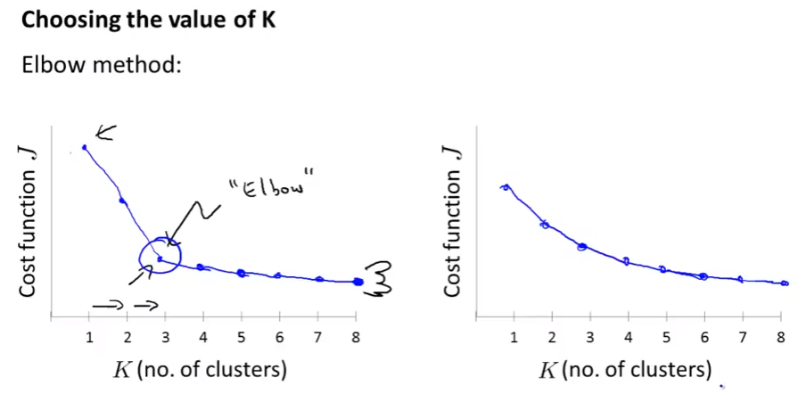
• If $k=5$ have bigger J than $k=3$ then k-means got stuck in a bad local minimum. You should try re-running k-means with multiple random initializations.
• Choose the number of clusters depend on later/downstream purpose (choose the size of T-shirt, 3 or 5 for example).

Dimensionality reduction

• Motivation: data compression + data visualization
• Househole’s note.

Data compression

• Speeds up algorithms + Reduces space used by data for them.
  • If all points in 2D lay on 1 straight line, we can reduce them to 1D cases. The same for 3D to 2D

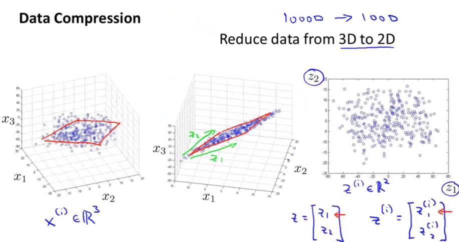
Data Visualization

• We want to reduce dimension to 2 or 3 so that we can visualize the data.

Principal component analysis (PCA)

PCA formulation

• Househole’s note.
• For the problem of dimensionality reduction the most commonly used algorithm is PCA
• For example, we want to find a line to translate 2D to 1D: all data point projected to this line should be small. The vector of this line is what we wanna find.
• You should normally do mean normalization and feature scaling (see again) on your data before PCA
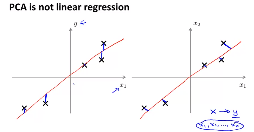
• PCA is not linear regression!!: PCA lấy error là các projection trong khi LG lấy error là sự sai lệch (theo y)
  • Below photo comapre pca (right) and linear regression (left).
  • LR has y to compare while PCA has no y, every x has equal role.

  

PCA algorithm

• How to use PCA for yourself + and how to reduce dimension for your data.
• Data preprocessing: feature scaling/mean normalization
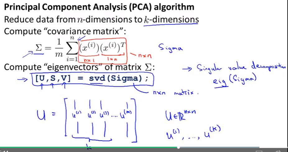
• svd in matlab/octave = “singular value decomposition” or eig function with the same function (svd is more numerically stable than eig)
  • Compute covariance matrix $\Sigma$
  • Compute Eigenvectors of matrix $\Sigma$

  

  • face Covariance matrix

    In probability theory and statistics, a covariance matrix is a matrix whose element in the $i, j$ position is the covariance between the i-th and j-th elements of a random vector.

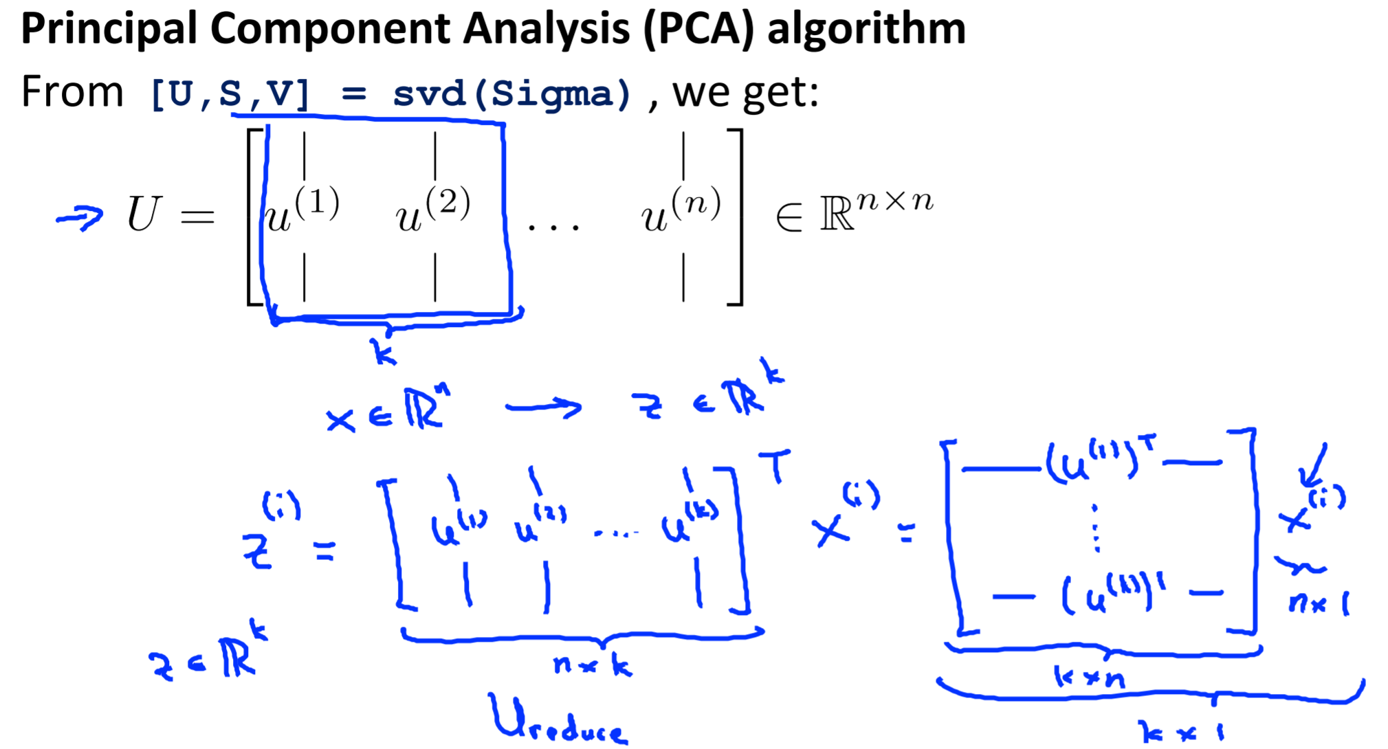
  • After having U, just take first k column if we wanna k dimension from n

  

• Algorithm:

  

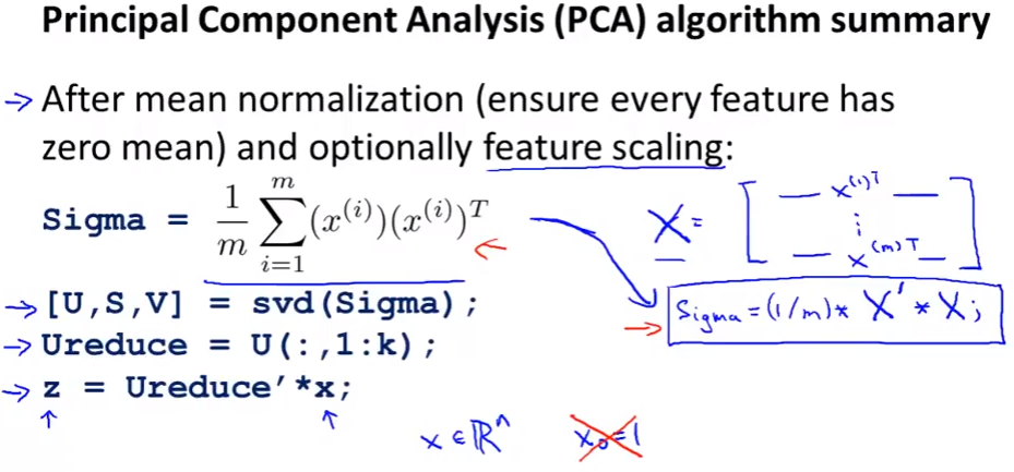
Applying PCA

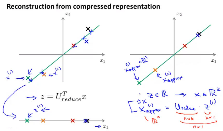
Reconstruction from compressed representation

From z back to x: 2D back to 1D for example,

Choosing the number of principal components

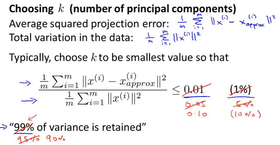
Choo k from 1 to the one get the fraction less than 0.001.

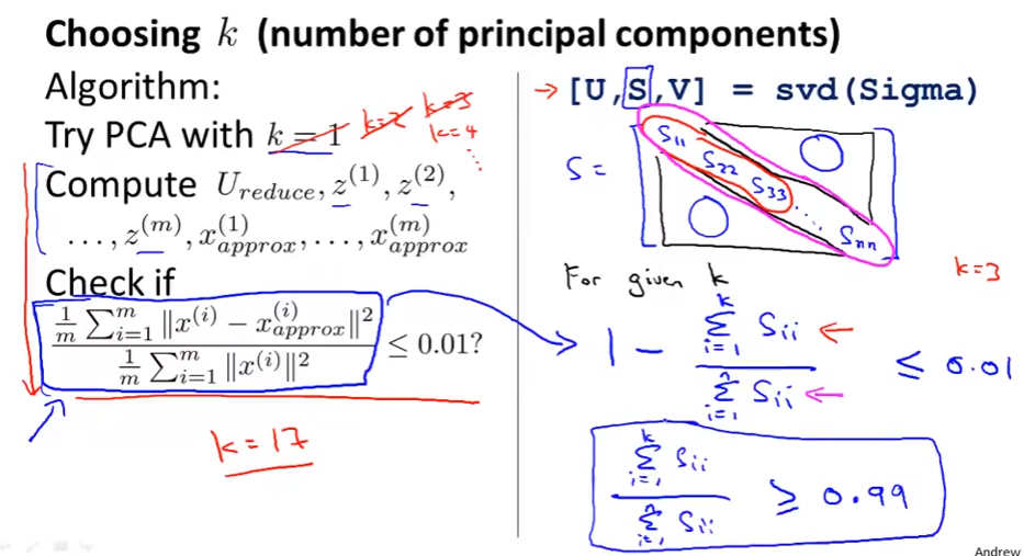
The numerator is small: we lose very little information in the dimensionality reduction, so when we decompress we regenerate the same data.

Advice for applying PCA

• Andrew uses PCA very often
• Defined by PCA only on the training set
  • And then use those obtained parameters to the Cross validation data and test set
• A bad use of PCA: Use it to prevent over-fitting –> Better to use regularization
• Always use normal approach (without PCA) to solve a problem, if you CANNOT DO MORE, then think about adding PCA.

Programming assignment

K-means Clustering

• The K-means algorithm is a method to automatically cluster similar data examples together.

• K-means algorithm is as follows

  % Initialize centroids
  centroids = kMeansInitCentroids(X, K);
  for iter = 1:iterations
    % Cluster assignment step: Assign each data point to the
    % closest centroid. idx(i) corresponds to cˆ(i), the index
    % of the centroid assigned to example i
    idx = findClosestCentroids(X, centroids);
    % Move centroid step: Compute means based on centroid
    % assignments
    centroids = computeMeans(X, idx, K);
  end
  

• Size: $X\in \mathbb{R}^{m\times n}$, $K\in \mathbb{R}$, centroids $\in \mathbb{R}^{K\times n}$, $c\in \mathbb{R}^{m\times 1}$ (idx is c)
  • $m$ examples, $n$ features

• File findClosestCentroids.m

  for i=1:size(X,1)
        min = 100; % initial
        for k=1:K
            if norm(X(i,:)-centroids(k,:)) < min
                    min = norm(X(i,:)-centroids(k,:));
                    min_idx = k;
            end
        end
        idx(i,1) = min_idx;
  end
  

• Computing centroid means: file computeCentroids.m

  for k=1:K
        idxCk = find(idx == k); % index of all X that corresponding to centroid k
        centroids(k,:) = sum(X(idxCk,:))/size(idxCk,1);
  end
  

• File kMeansInitCentroids.m (Random initialization)

  % Initialize the centroids to be random examples
  % Randomly reorder the indices of examples
  randidx = randperm(size(X, 1));
  % Take the first K examples as centroids
  centroids = X(randidx(1:K), :);
  

Image compression with K-means

Check the guide in ex7.pdf, page 7.

In this exercise, you will use the K-means algorithm to select the 16 colors that will be used to represent the compressed image. Concretely, you will treat every pixel in the original image as a data example and use the K-means algorithm to find the 16 colors that best group (cluster) the pixels in the 3-dimensional RGB space. Once you have computed the cluster centroids on the image, you will then use the 16 colors to replace the pixels in the original image.

PCA

PCA consists of two computational steps:

• First, you compute the covariance matrix of the data.
• Then, you use Octave/MATLAB’s SVD function to compute the eigenvectors $U_1, U_2,\ldots,U_n$.

Before using PCA, it is important to first normalize the data by subtracting the mean value of each feature from the dataset, and scaling each dimension so that they are in the same range.

File pca.m

Sigma = 1/m * (X'*X);
[U, S, ~] = svd(Sigma);

Dimensionality Reduction with PCA

File projectData.m:

Ureduce = U(:,1:K);
Z = X*Ureduce;

File recoverData.m

Ureduce = U(:,1:K);
X_rec = Z*Ureduce';

Face Image Dataset

In this part of the exercise, you will run PCA on face images to see how it can be used in practice for dimension reduction.

For example, if you were training a neural network to perform person recognition (gven a face image, predict the identitfy of the person), you can use the dimension reduced input of only a 100 dimensions instead of the original pixels.