
ML Coursera 2 - w2: Linear Regression with Multiple Variables
Posted on 01/09/2018, in Machine Learning.This note was first taken when I learnt the machine learning course on Coursera.
Lectures in this week: Lecture 4, Lecture 5.
Multivariate Linear Regression
Multiple Features
Linear regression with multiple variables is also known as “multivariate linear regression”. We now introduce notation for equations where we can have any number of input variables.
- $x^{(i)}_j$ = value of feature j in the ith training example
- $x^{(i)}$ = the input (features) of the ith training example
- m = the number of training examples
- n = the number of features
The multivariable form of the hypothesis function accommodating these multiple features is as follows:
In order to develop intuition about this function, we can think about $\theta_0$ as the basic price of a house, $\theta_1$ as the price per square meter, $\theta_2$ as the price per floor, etc. $x_1$ will be the number of square meters in the house, $x_2$ the number of floors, etc.
Using the definition of matrix multiplication, our multivariable hypothesis function can be concisely represented as:
This is a vectorization of our hypothesis function for one training example; see the lessons on vectorization to learn more.
Remark: Note that for convenience reasons in this course we assume $x_{0}^{(i)} =1 \text{ for } (i\in { 1,\dots, m } )$. This allows us to do matrix operations with theta and x. Hence making the two vectors $\theta$ and $x^{(i)}$ match each other element-wise (that is, have the same number of elements: n+1).
Gradient descent for multiple variables
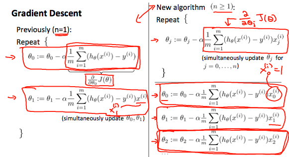
The gradient descent equation itself is generally the same form; we just have to repeat it for our ‘n’ features:
In other words:
The following image compares gradient descent with one variable to gradient descent with multiple variables:
GD in practice : Feature scaling
- If features have diff values, when we perform them on a plot, there may be very different on scale between axes! It may impact on the gradient descent!
- Feature scaling: An option is to divide to a maximum value, for example, $x \in \{1,\ldots, 2000\}$ can be scale to $\bar{x} \in \dfrac{\{1,\ldots,2000\}}{2000}$ so that we have the values are between $[-1,1]$. However, not used for range of $[-100,100]$ of bigger or $[-0.0001,0.0001]$ or smaller.
-
Another option is to use mean normalisation (Do not apply to $x_0$)
$$ \bar{x}_i = \dfrac{x_i - \mu_i}{\text{range of }x_i}, \quad \mu_i = \Sigma_i \frac{x_i}{m}. $$Then $-0.5 \le x_i \le 0.5$. For example, $x_i \in [30,50]$, then range of $x_i$ is 20.
GD in practice : Learning rate $\alpha$
- Debugging: How to make sure gradient descent works correctly?
- How to choose learning rate $\alpha$?
Methods
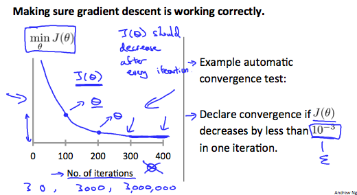
- Examine the convergence of $\min_{\theta} J(\theta)$ w.r.t the number of iterations.
-
Declare convergence if $J(\theta)$ decreases by less than $10^{-1}$ in one iteration.
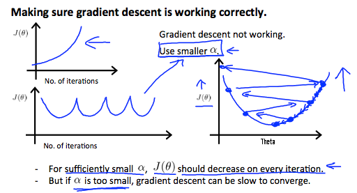
- If $J(\theta)$ increase, use smaller $\alpha$ (can prove it mathematically).
- But if $\alpha$ is too small, gradient descent can be slow to converge.
-
Try $\alpha$ with $0.001, 0.003, 0.01, 0.03, 0.1, 0.3, 1,\ldots $ (try a little bit and get the good value of $\alpha$)
Features and Polynomial Regression
We can improve our features and the form of our hypothesis function in a couple different ways. We can combine multiple features into one. For example, we can combine $x_1,x_2$ into a new feature called $x_3 = x_1x_2$.
We can change the behavior or curve of our hypothesis function by making it a quadratic, cubic or square root function (or any other form).
For example, if our hypothesis function is $h_\theta(x) = \theta_0 + \theta_1 x_1$ then we can create additional features based on $x_1$ to get the quadratic function $h_\theta(x) = \theta_0 + \theta_1 x_1 + \theta_2 x_1^2$ or the cubic function $h_\theta(x) = \theta_0 + \theta_1 x_1 + \theta_2 x_1^2 + \theta_3 x_1^3$
In the cubic version, we have created new features $x_2$ amd $x_3$ where $x_2=x_1^2, x_3=x_1^3$ . To make it a square root function, we could do: $h_\theta(x) = \theta_0 + \theta_1 x_1 + \theta_2 \sqrt{x_1}$
One important thing to keep in mind is, if you choose your features this way then feature scaling becomes very important.
For example, if $x_1$ has range 1-10, then $x_1^2$ has range 1-100, $x_1^3$ has range 1-1000.
Computing Parameters Analytically
Normal equation
- Normal equation: method to solve for $\theta$ analytically (instead of solve it by iteration)
-
Example, m examples, n feautures then the design matrix X will be
$$ m \times (n+1) $$The first column is the supposed feature whose all values are equal to 1.
-
the value of $\theta$ that minimize your cost function $J(\theta)$
$$ \theta = (X^TX)^{-1}X^Ty $$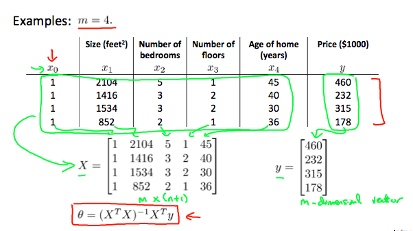
- In this case (normal equation, analytically), feature scaling seems not to be important!
- But in gradient descent, feature scaling is important!
- If number of features is less than 10000, use normal equation.. If bigger than that, change to iterative process.
| Gradient Descent | Normal Equation |
|---|---|
| Need to choose alpha | No need to choose alpha |
| Needs many iterations | No need to iterate |
| $O(kn^2)$ | $O (n^3)$, need to calculate inverse of $X^TX$ |
| Works well when n is large | Slow if n is very large |
Normal equation noninvertibility
When implementing the normal equation in octave we want to use the pinv function rather than inv. The pinv function will give you a value of $\theta$ even if $X^TX$ is not invertible.
If $X^TX$ is noninvertible, the common causes might be having :
- Redundant features, where two features are very closely related (i.e. they are linearly dependent)
- Too many features (e.g. $m \le n$). In this case, delete some features or use “regularization” (to be explained in a later lesson).
Solutions to the above problems include deleting a feature that is linearly dependent with another or deleting one or more features when there are too many features.
Quiz’s answers
-
Question 1:
where $\mu = \dfrac{\sum_i x^{(i)}_1}{n} = 81 $ and $range = 94-69=25$.
- Question 2: Using a bigger $\alpha$ because $J(\theta)$ decreases slowly (and keep decreasing).
- Question 3: Size of $X$ is $m\times (n+1)$ where $m= $ numer of training examples, $n= $ number of features. Then, size of $X$ is $28\times 5$, size of $X^T$ is $5\times 28$, $y$ has size of $m\times 1$. Finally, we get size of $\theta$ is $5\times 1$.
- Question 4: Remember that, in practice, if number of features is less than 10000, use normal equation.
- Question 5: feature scaling is important in gradient descent, not in normal equation.
Octave / Matlab
I have already known about matlab, so this part of note contains not too much information from the course.
- Note on operators:
hist,eye,rand. - Moving data, notice on these:
pwd,load,who,whos,save,A(:)puts all elements into a single vector
- Computing on data:
[val, ind] = max(A)max(A,[],2)flipud
- Plotting data:
imagesc - Control statement
- Vectorization: make your codes run more quickly.
Exercice de programmation: Linear Regression
LR with one variable (required)
-
warmUpExercise.m : nothing to say.
A = eye(5); -
plotData.m: nothing to say, just using the
plotcommand.plot(x, y, 'rx', 'MarkerSize', 10); % plot the data ylabel('Profit in $10,000'); % Set the y-axis label xlabel('Population of City in 10,000s'); % Set the x-axis label -
computeCost.m: follows the formula of cost function
Note that, there is some confusion in the notations given in the talk of Ng about the dimension of $X$.
J = 1/(2*m)*sum((X*theta - y).^2); -
gradientDescent.m: follows the formula of Gradient Descent for linear regression given at the end of Week 1.
Notice that, $\theta_0, \theta_1$ are computed simultaneously!!
thetaOld = theta; % prevent the changes theta(1,1) = thetaOld(1,1) - alpha * (1/m) * sum(X*thetaOld - y); theta(2,1) = thetaOld(2,1) - alpha * (1/m) * dot((X*thetaOld - y),X(:,2)); -
The code for visualizing $J(\theta_0,\theta_1)$
fprintf('Visualizing J(theta_0, theta_1) ...\n') % Grid over which we will calculate J theta0_vals = linspace(-10, 10, 100); theta1_vals = linspace(-1, 4, 100); % initialize J_vals to a matrix of 0's J_vals = zeros(length(theta0_vals), length(theta1_vals)); % Fill out J_vals for i = 1:length(theta0_vals) for j = 1:length(theta1_vals) t = [theta0_vals(i); theta1_vals(j)]; J_vals(i,j) = computeCost(X, y, t); end end % Because of the way meshgrids work in the surf command, we need to % transpose J_vals before calling surf, or else the axes will be flipped J_vals = J_vals'; % Surface plot figure; surf(theta0_vals, theta1_vals, J_vals) xlabel('\theta_0'); ylabel('\theta_1'); % Contour plot figure; % Plot J_vals as 15 contours spaced logarithmically between 0.01 and 100 contour(theta0_vals, theta1_vals, J_vals, logspace(-2, 3, 20)) xlabel('\theta_0'); ylabel('\theta_1'); hold on; plot(theta(1), theta(2), 'rx', 'MarkerSize', 10, 'LineWidth', 2); -
Now, you can submit your work by typing
submit().
LR with multiple variables (optional)
-
featureNormalize.m: We need to store mean and standard deviation after nomalizing step because we will use them to nomalize a “new” data test.
mu = mean(X); % mean of features sigma = std(X); % standard deviation X_norm = (X - mu) ./ sigma; -
computeCostMulti.m: code generated in this case can be used for
ex1also.J = 1/(2*m) * (X*theta - y)' * (X*theta - y); -
gradientDescentMulti.m: code generated in this case can be used for
ex1also.n = size(X,2); % number of features theta = theta - alpha * (1/m) * transpose(dot(repmat(X*theta - y,1,n),X,1)); -
ex1_multi.m: There are two notes. (1) if using feature nomalize, it’s necessary to nomalize X_test before finding the price. (2) If using normal equation, no need to use normalization.
% using feature normalization
% (choose alpha = 0.03 to get better resutl)
x_test = [1650 3];
x_test = (x_test - mu) ./ sigma;
x_test = [1, x_test];
price = x_test * theta;
% using normal equation
x_test = [1 1650 3];
price = x_test * theta;