This note was first taken when I learnt the machine learning course on Coursera.
Lectures in this week: Lecture 12.

error From this note, I see that this note of Alex Holehouse is really detailed so that I can use it for the future reference. I don’t have enough time for noting as previous note.

• So far, we’ve seen a range of different algorithms
  • With supervised learning algorithms - performance is pretty similar. What matters more often is:
    • The amount of training data
    • Skill of applying algorithms
• One final supervised learning algorithm that is widely used - support vector machine (SVM)
  • Compared to both logistic regression and neural networks, a SVM sometimes gives a cleaner way of learning non-linear functions
  • Later in the course we’ll do a survey of different supervised learning algorithms

Large margin classification

Optimization objective

• Alternative view of logistic regression: we see the cost function is a function of $z=X\Theta$.
• To build a SVM we must redefine our cost functions
  • Instead of a curved line create two straight lines (magenta) which acts as an approximation to the logistic regression $y = 1$ function
  • So here we define the two cost function terms for our SVM graphically

  

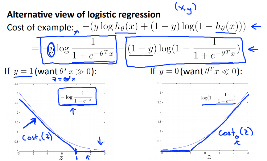  $$ \begin{align} cost_0 &= -\log(1-\dfrac{1}{1+e^{-z}}) \\ cost_1 &= -\log(\dfrac{1}{1+e^{-z}}) \end{align} $$

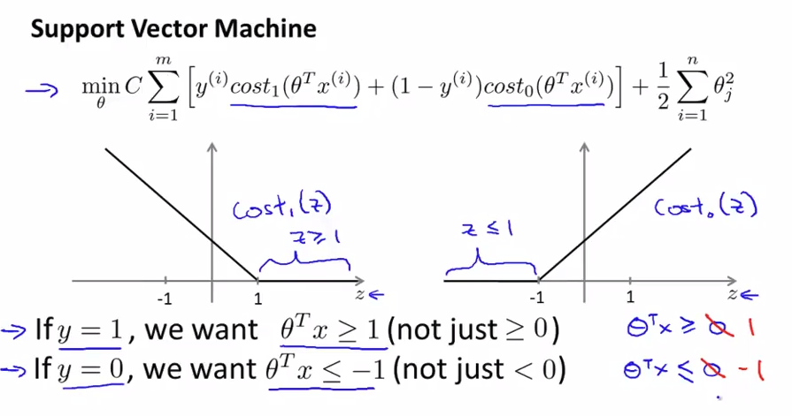
• So we get (new SVM cost function)

  $$\min \dfrac{1}{m}\left[ \sum_{i=1}^m y^{(i)} cost_1(\Theta^Tx^{(i)}) + (1-y^{(i)})cost_0(\Theta^Tx^{(i)}) \right] + \dfrac{\lambda}{2m}\sum_{i=1}^n \theta^2_j$$

• We use another notation to minimize problem

  $$\min_{\Theta} C \sum_{i=1}^m \left[ \sum_{i=1}^m y^{(i)} cost_1(\Theta^Tx^{(i)}) + (1-y^{(i)})cost_0(\Theta^Tx^{(i)}) \right] + \dfrac{1}{2}\sum_{i=1}^n \theta^2_j$$
• Unlike logistic, $h_{\theta}(x)$ doesn’t give us a probability, but instead we get a direct prediction of 1 or 0 (as mentioned before)

Large margin intuition

• Logistic regression only need $X\Theta\ge 0$ to get $h=1$ or $X\Theta <0$ to get $0$. SVM gives us a clearer way ($X\Theta \ge 1$ and $X\Theta <-1$ respectively).

  

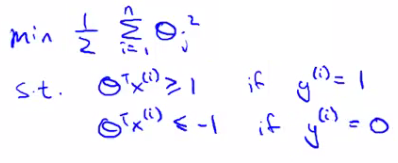
• Consider a case in which $C$ very huge, we need to choose $\Theta$ such that $A=0$ ($A$ in $CA+B$).
  • If $y1$, we need to find $\Theta$ such that $X\Theta \ge 1$
  • If $y=0$, find $\Theta$ such that $X\Theta <-1$

• When $CA=0$, the minimization problem becomes,

  

• Mathematically, that black line has a larger minimum distance (margin) from any of the training examples

  

Mathematics behind large classification

Kernels

Kernels I

• That a hypothesis computes a decision boundary by taking the sum of the parameter vector multiplied by a new feature vector f, which simply contains the various high order x terms

  $$\begin{align} h_{\theta}(x) &= \theta_0 + \theta_1f_1 + \theta_2 + \ldots, \\ f_1 &= x_1, f_2 = x_1x_2, \ldots \end{align}$$

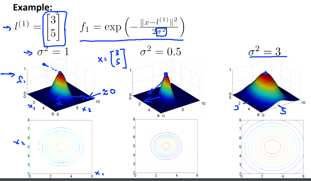
• We choose landmarks $l^{(1)}, l^{(2)}, \ldots$ and then using the similarity (kernel) between $x$ and each landmark $l^{(i)}$.

  $$ \begin{align} \text{similarity} = k(x,l^{(i)}) &= \exp\left( -\dfrac{\Vert x-l^{(i)}\Vert^2}{2\sigma^2} \right) \\ f_i &:= \text{similarity}(x,l^{(i)}). \end{align} $$
  • $\sigma$: standard deviation
  • $\sigma^2$: variance.
  • $\Vert \cdot \Vert$: Euclidean distance
  $$\Vert x-l^{(i)}\Vert^2 = \sum_{j=1}^n (x_j-l_j^{(i)})$$
  • There are many kernels, above def of similarity is Gaussian kernel.

  

  • We call $f$ landmark also!

Kernels II

• Where do we get the landmarks from?
• For each example place a landmark at exactly the same location
  • Given $m$ examples of $n$ features $(x^{(i)}, y^{(i)})$ for $i=1,m$.
  • Choose landmarks: $l^{(i)} = x^{(i)}$ where $i=1,m$.
  • We will build $m$ landmark $f^{(i)}$, each of them is built from
  $$f_k^{(i)} = k(x^{(i)}, l^{(k)}), \text{ for } k=1,m.$$
• Note that $m$ input elements $x^{(i)}$ becomes $m+1$ landmarks $f$ ($f^{0} = 1$)
• $\Theta$ now becomes $\Theta \in \mathbb{R}^{(m+1)\times 1}$.
• $f\in \mathbb{R}^{(m+1)}$ also.
• Predict $1$ if $\Theta^Tf \ge 0$

• SVM learning algorithm

  $$ \min_{\Theta} C\sum_{i=1}^m \left( y^{(i)} cost_1 (\Theta^Tf^{(i)}) + (1-y^{(i)})cost_0(\Theta^Tf^{(i)})\right) + \dfrac{1}{2}\sum_{j=1}^m\phi_j^2, \quad (n=m \text{ in this case}) $$
• We minimize using $f$ as the feature vector instead of $x$
• $m=n$ because number of features is the number of training data examples we have.
• It’s really expensive because there may be a lot of features (= number of training examples). It's good to use shelf software to minimize this function instead. DON’T write your own software to do that!!
• Variance vs Bias trade-off
  • Large $C$ ($\frac{1}{\lambda}$): low bias, high variance $\Rightarrow$ overfitting.
  • Small C gives a hypothesis of high bias low variance $\Rightarrow$ underfitting
  • Large $\sigma^2$: f features vary more smoothly - higher bias, lower variance
  • Small $\sigma^2$: f features vary unexpectedly - low bias, high variance

SVMs in practice

Using an SVM

• Don’t write yourown codes to linearize the SVM, use already-writen library such as liblinear, libsvm, …
  • Choice of $C$
  • Choice of kernel (similarly functions)
    • No kernel (“linear kernel”, use $X\Theta$)
    • Gaussian kernel (above): need to choose $\sigma^2$
• Do perform feature scaling before using Gaussian kernel
• Not all similarity functions you develop are valid kernels $\Rightarrow$ Must satisfy Merecer’s Theorem to make sure SVM packages’ optimizations run correctly, and do not diverge.
• Polynomial kernel:
  • use when $x$ and $l$ are both strictly non-negative
  • People not use this much.
  • parameters: $const$ and $degree$
  $$k(x,l) = (X^Tl + const)^{degree}$$
• Other kernels: string kernel (input data using texts, string,…), chi-square kernel, histogram intersection kernel,…
• Remember: choose whatever kernel performs best on cross-validation data

Multiclass classification

• Many packages have built in multi-class classification packages
• Otherwise use one-vs all method
• Not a big issue

Logistic regression vs. SVM

• If n (features) is large vs. m (training set)
  • Feature vector dimension is 10 000
  • Training set is 10 - 1000
  • Then use logistic regression or SVM with a linear kernel
• If n is small and m is intermediate
  • n = 1 - 1000
  • m = 10 - 10 000
  • Gaussian kernel is good
• If n is small and m is large
  • n = 1 - 1000
  • m = 50 000+
  • SVM will be slow to run with Gaussian kernel
  • In that case
    • Manually createMul(Dclass*classifica(on or add more features
    • Use *logistic Mul(Dclassclassifica(onregression of SVM with a linear kernel** Mul(Dclass*classifica(on
• Logistic regressionMul(Dclass*classifica(on and SVM with a linear kernel are pretty similar (performance, works)
• SVM has a convex optimization problem - so you get a
• Neural network likely to work well for most of these settings, but may be slower to train.

Programming Assignment

SVM

• A large $C$ parameter tells the SVM to try to classify all the examples correctly. $C$ plays a role similar to $\frac{1}{\lambda}$ , where $\lambda$ is the regularization parameter that we were using previously for logistic regression.

  settings_backup_restore See again Regularized logistic regression.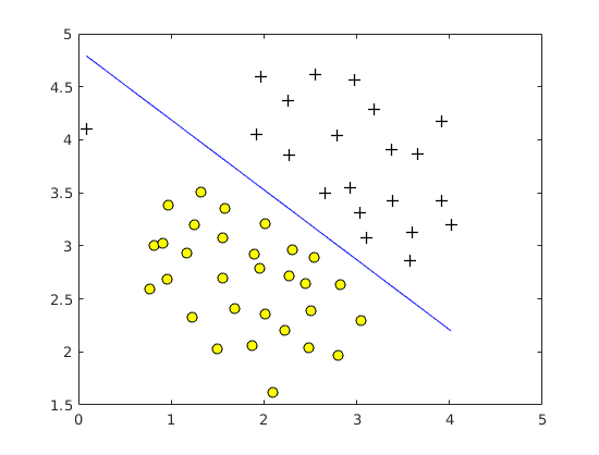

  $C=1$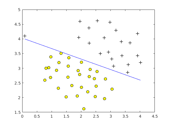

  $C=100$

• Most SVM software packages (including svmTrain.m) automatically add the extra feature $x_0 = 1$ for you and automatically take care of learning the intercept term $\theta_0$. So when passing your training data to the SVM software, there is no need to add this extra feature $x_0 = 1$ yourself.

SVM with Gaussian Kernels

• To find non-linear decision boundaries with the SVM, we need to first implement a Gaussian kernel.
• You can think of the Gaussian kernel as a similarity function that measures the “distance" between a pair of examples $(x^{(i)}, x^{(j)})$. The Gaussian kernel is also parameterized by a bandwidth parameter, $\sigma$, which determines how fast the similarity metric decreases (to 0) as the examples are further apart.

• The Gaussian kernel function defined as

  $$K_{Gaussian}(x^{(i)}, x^{(j)}) = \exp\left( -\dfrac{\Vert x^{(i)} - x^{(j)} \Vert^2}{2\sigma^2} \right) = \exp\left( -\dfrac{ \sum_{k=1}^n(x^{(i)} - x^{(j)})^2 }{2\sigma^2} \right)$$

• File gaussianKernel.m

  sim = exp( -(norm(x1-x2))^2/(2*sigma^2) );
  

Example Dataset 3

File dataset3Params.m

range = [0.01, 0.03, 0.1, 0.3, 1, 3, 10, 30];
predictionErrMin = 100000; % initial

for i=1:size(range,2)
   for j=1:size(range,2)
       model= svmTrain(X, y, range(i), @(x1, x2) gaussianKernel(x1, x2, range(j))); 
       predictions = svmPredict(model, Xval);
       predictionErr = mean(double(predictions ~= yval));
       if predictionErr < predictionErrMin
           predictionErrMin = predictionErr;
           C = range(i);
           sigma = range(j);
       end
   end
end

Spam Classification

• You need to convert each email into a feature vector $x\in \mathbb{R}^n$. The following parts of the exercise will walk you through how such a feature vector can be constructed from an email.

Preprocessing Emails

• One method often employed in processing emails is to “normalize” these values, so that all URLs are treated the same, all numbers are treated the same, etc.
  • we could replace each URL in the email with the unique string httpaddr to indicate that a URL was present.
• Usually, we do:
  • Lower-casing: convert entire email to lowercase.
  • Stripping HTML: All HTML tags are removed from the emails.
  • Normalizing URLs: All URLs are replaced with the text httpaddr
  • Normalizing Email Addresses: with the text emailaddr.
  • Normalizing Numbers: number.
  • Normalizing Dollars: All dollar signs ($) are replaced with the text dollar.
  • Word Stemming: “discount”, “discounts”, “discounted” and “discounting” replace by discount
  • Removal of non-words: Non-words and punctuation have been removed. all tabs, spaces, newlines becomes 1-space character.

Vocabulary List

• Our vocabulary list was selected by choosing all words which occur at least a 100 times in the spam corpus, resulting in a list of 1899 words. In practice, a vocabulary list with about 10,000 to 50,000 words is often used.
• Given the vocabulary list, we can now map each word in the preprocessed emails (e.g., Figure 9) into a list of word indices that contains the index of the word in the vocabulary list.
  • If the word exists, you should add the index of the word into the word indices variable.
  • If the word does not exist, and is therefore not in the vocabulary, you can skip the word.

• File processEmail.m

  for i=1:length(vocabList)
      if strcmp(str, vocabList{i})
          word_indices = [word_indices; i]; 
      end
  end
  

Extracting Features from Emails

• You will now implement the feature extraction that converts each email into a vector in $\mathbb{R}^n$.
• $n=$ number of words in vocabulary list.
• $x_i\in {0,1}$ for an email corresponds to whether the i-th word in the dictionary occurs in the email.

• File emailFeatures.m

  x(word_indices)=1;