This note was first taken when I learnt the IBM Data Professional Certificate course on Coursera.

Week 4: Clustering

What’s clustering?

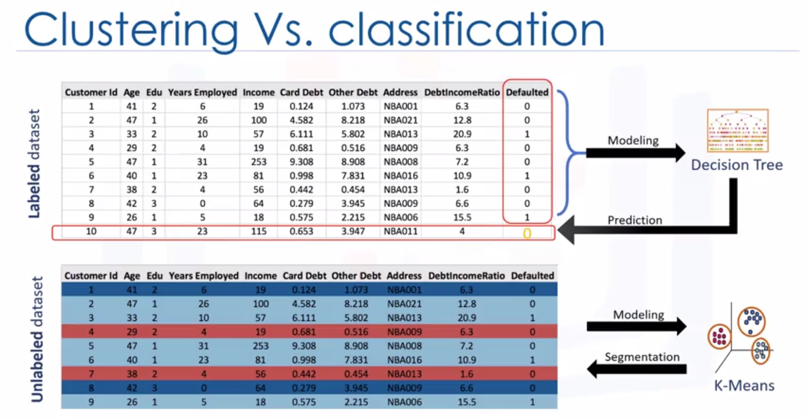
• The important requirement is to use the available data to understand and identify how customers are similar to each other. Let’s learn how to divide a set of customers into categories, based on characteristics they share.
• Clustering can group data only unsupervised, based on the similarity of customers to each other.
• Having this information would allow your company to develop highly personalized experiences for each segment.
• Clustering means finding clusters in a dataset, unsupervised.
• What’s difference between clustering and classification?
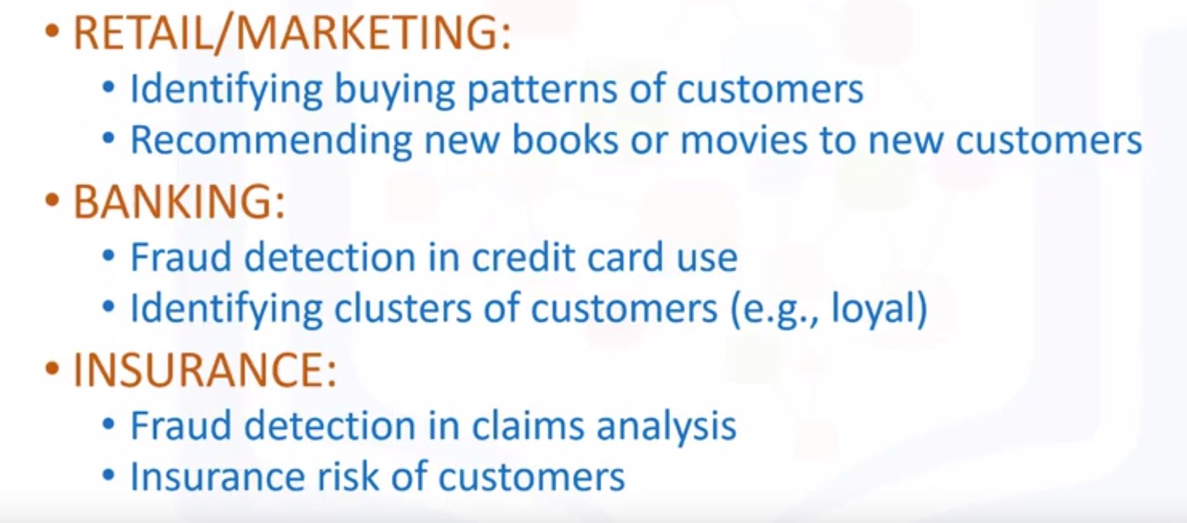
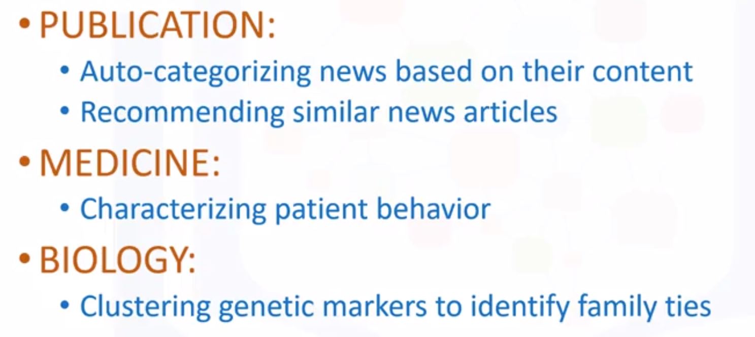
• Application of clustering

  

  

• Why clustering?
  • Exploratory data analysis
  • Summary generation
  • Outlier detection
  • Finding duplicates
  • Pre-processing steps
• Clustering algorithms
  • Partitioned-based clustering
    • Relatively efficient
    • eg. K-means, k-median, fuzzy c-means
    • used for medium or large size databases
  • Hierarchical clustering
    • produces trees of clusters
    • eg. agglomerative, divisive
    • very intuitive
    • good for small size dataset
  • Density-based clustering
    • produces arbitary shaped clusters
    • eg. DBSCAN
    • used for special cluster or there is noise in your dataset

k-Means Clustering

The lab of K-means. This is another lab from course 9.

• K-Means can group data only unsupervised based on the similarity of customers to each other.
  • Partitioning clustering
  • K-means divides the data into non-overlapping subsets (clusters) without any cluster-internal structure
  • Examples within a cluster are very similar
  • Examples across different clusters are very different
• Onjective of k-means
  • To form clusters in such a way that similar samples go into a cluster, and dissimilar samples fall into different clusters.
  • To minimize the “intra cluster” distances and maximize the “inter-cluster” distances.
  • To divide the data into non-overlapping clusters without any cluster-internal structure
• k-means clustering - initialize k
  1. Initialize k=3 centrois randomly
     • Choose randomly 3 points in our data points.
     • Choose randomly 2 points (not in our data points)
  2. Find the distance to these centroids from each of data points.
  3. Assign each point to the closest centroid -> use distance matrix
  4. However, because we choose randomly the centroids, the SSE (sum of squared differences between each point and its centroid) is big
  $$SSE = \Sigma (x_i-c_j)^2$$
  1. Move the centroid to the mean of each cluster
  2. Go back to step 2 and repeat until there are no more changes.
  3. Above algorithm leads to local optimal (not guarantee about global optimal)
  4. Run the whole process multiple times with different starting conditions (the algorithm is quite fast)
• Accuracy of k-means
  • elbow method:
    • If we increase K, the mean distances are always deacrease -> cannot increase K forever
    • But, there is an “elbow”, the decreasing is much. We choose the K at this elbow!

Hierarchical Clustering

The lab of Hierarchical Clustering

• Hierarchical clustering algorithms build a hierarchy of clusters where each node is a cluster consisting of the clusters of its daughter nodes.
• Strategies for hierarchical clustering generally fall into two types,
  • divisive (phân tán ra) : dividing the cluster, it’s top-down.
  • agglomerative (tích tụ vào) : amass or collect things, it’s bottom-up -> more popular!
• Hierarchical clustering is illustrated by dendrogram (sơ đồ nhánh).
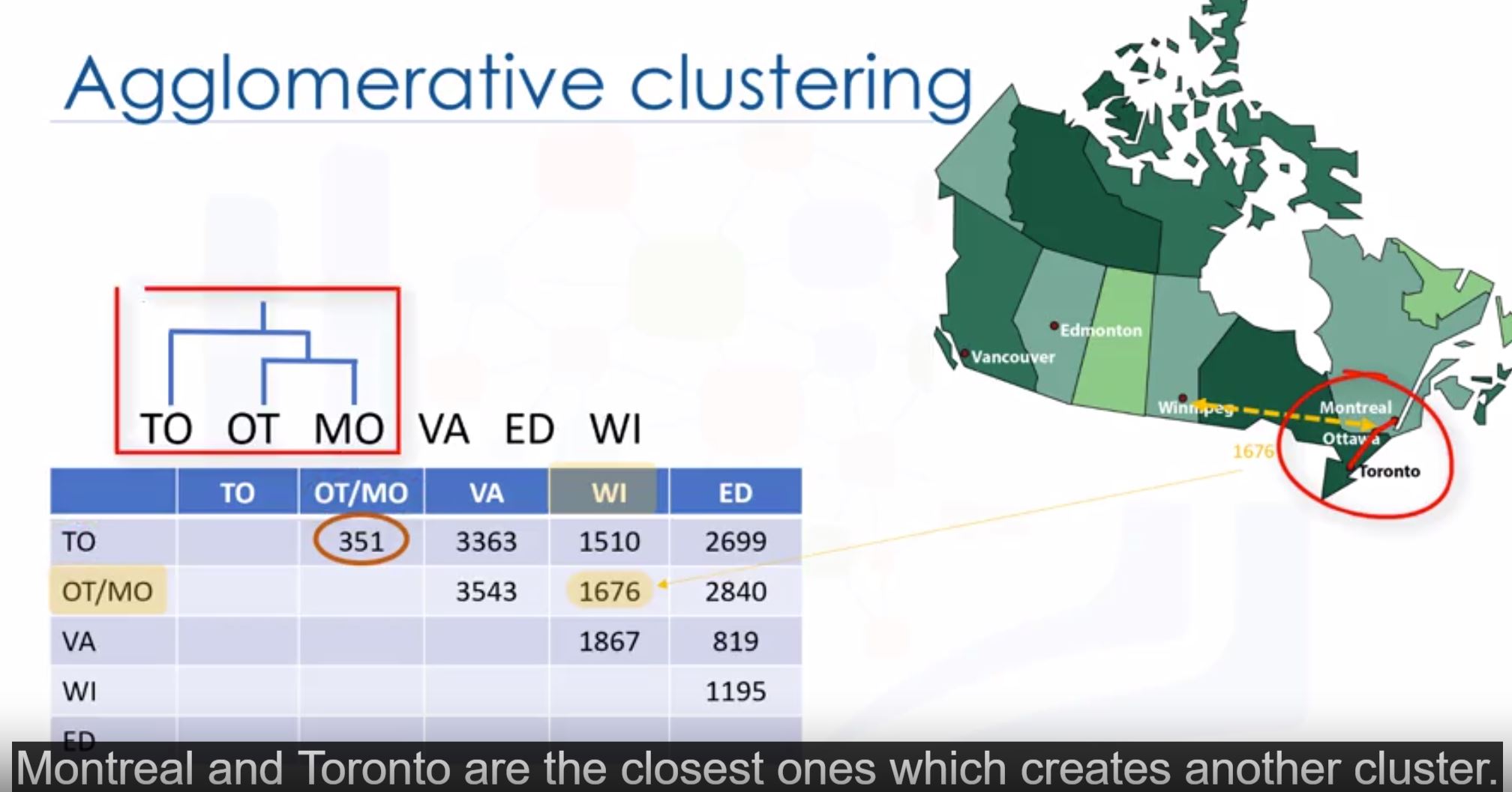
• Agglomerative algorithm
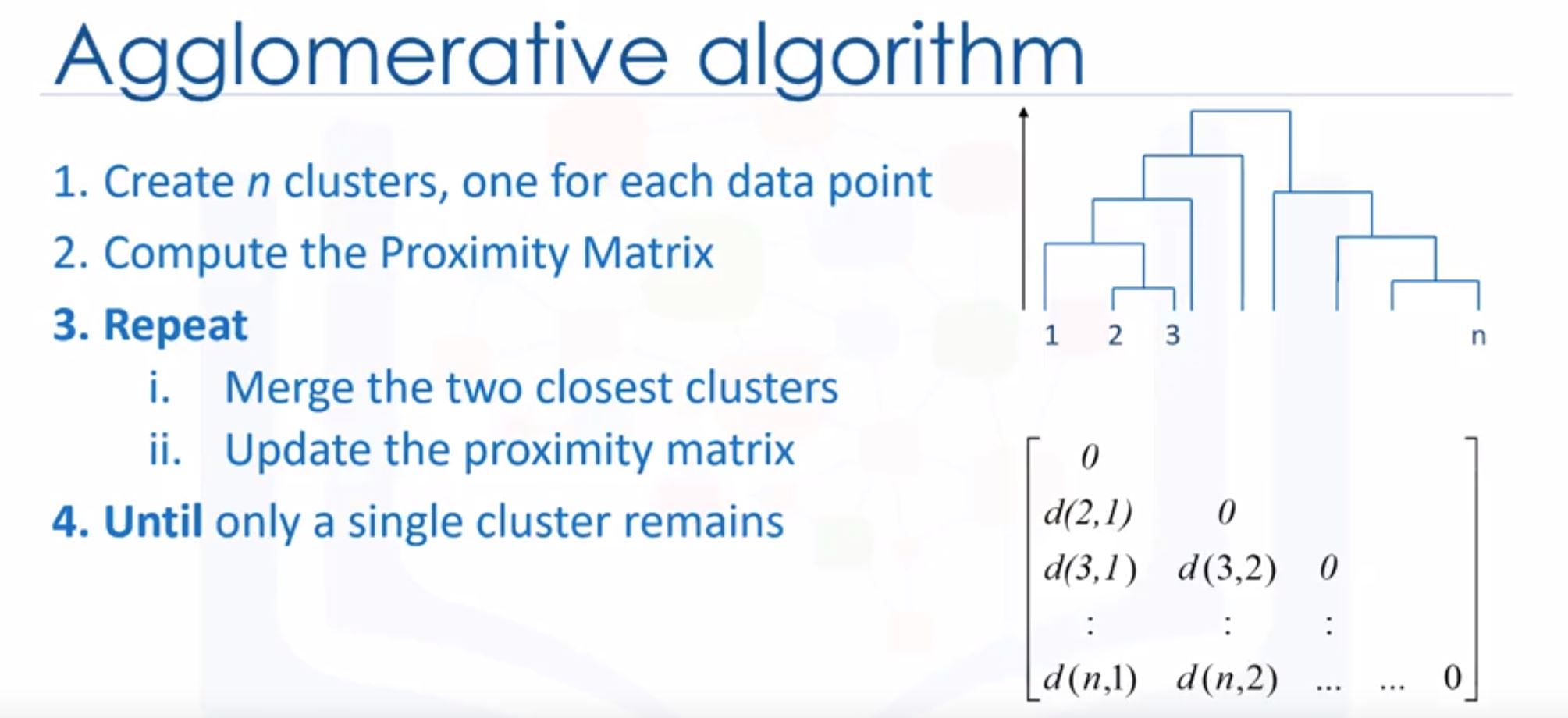
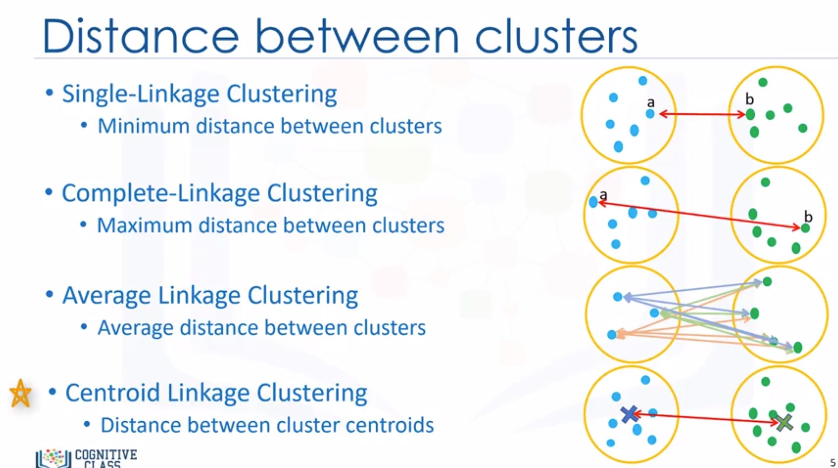
• To calculate distance between clusters:
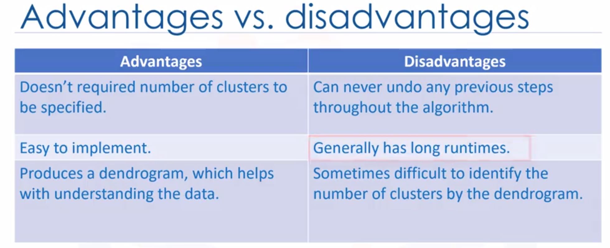
• Hierarchical clustering has longer runtimes than K-means!
• Advantages vs disavadtages
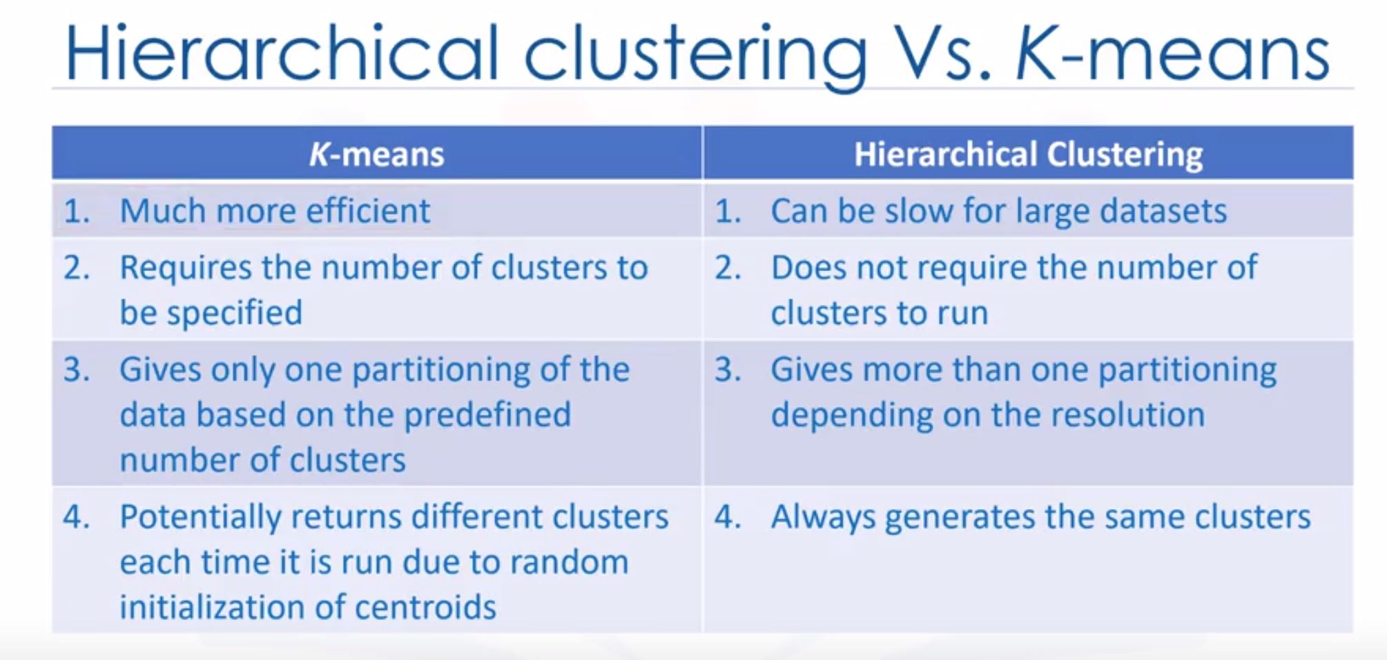
• Hierarchical clustering vs K-means

Hierarchical Clustering (lab)

The lab of Hierarchical Clustering

Generating Random Data

from sklearn.datasets.samples_generator import make_blobs
X1, y1 = make_blobs(n_samples=50, centers=[[4,4], [-2, -1], [1, 1], [10,4]], cluster_std=0.9)
# cluster_std: The standard deviation of the clusters. The larger the number, the further apart the clusters
#   Choose a number between 0.5-1.5

Plot the data

plt.scatter(X1[:, 0], X1[:, 1], marker='o') 

Agglomerative Clustering

from sklearn.cluster import AgglomerativeClustering
agglom = AgglomerativeClustering(n_clusters = 4, linkage = 'average')
agglom.fit(X1,y1)

Find the distance matrix

from scipy.spatial import distance_matrix
dist_matrix = distance_matrix(X1,X1) 

Hierarchical clustering

from scipy.cluster import hierarchy
Z = hierarchy.linkage(dist_matrix, 'complete')

Save the dendrogram to a variable called dendro

dendro = hierarchy.dendrogram(Z)

Check the lab to know how to use scipy to calculate distance matrix.

Density-based Clustering (DBSCAN Clustering)

The lab of Density-Based Clustering

• Works based on density of objects.
• When applied to tasks with arbitrary shaped clusters or clusters within clusters, traditional techniques might not be able to achieve good results.
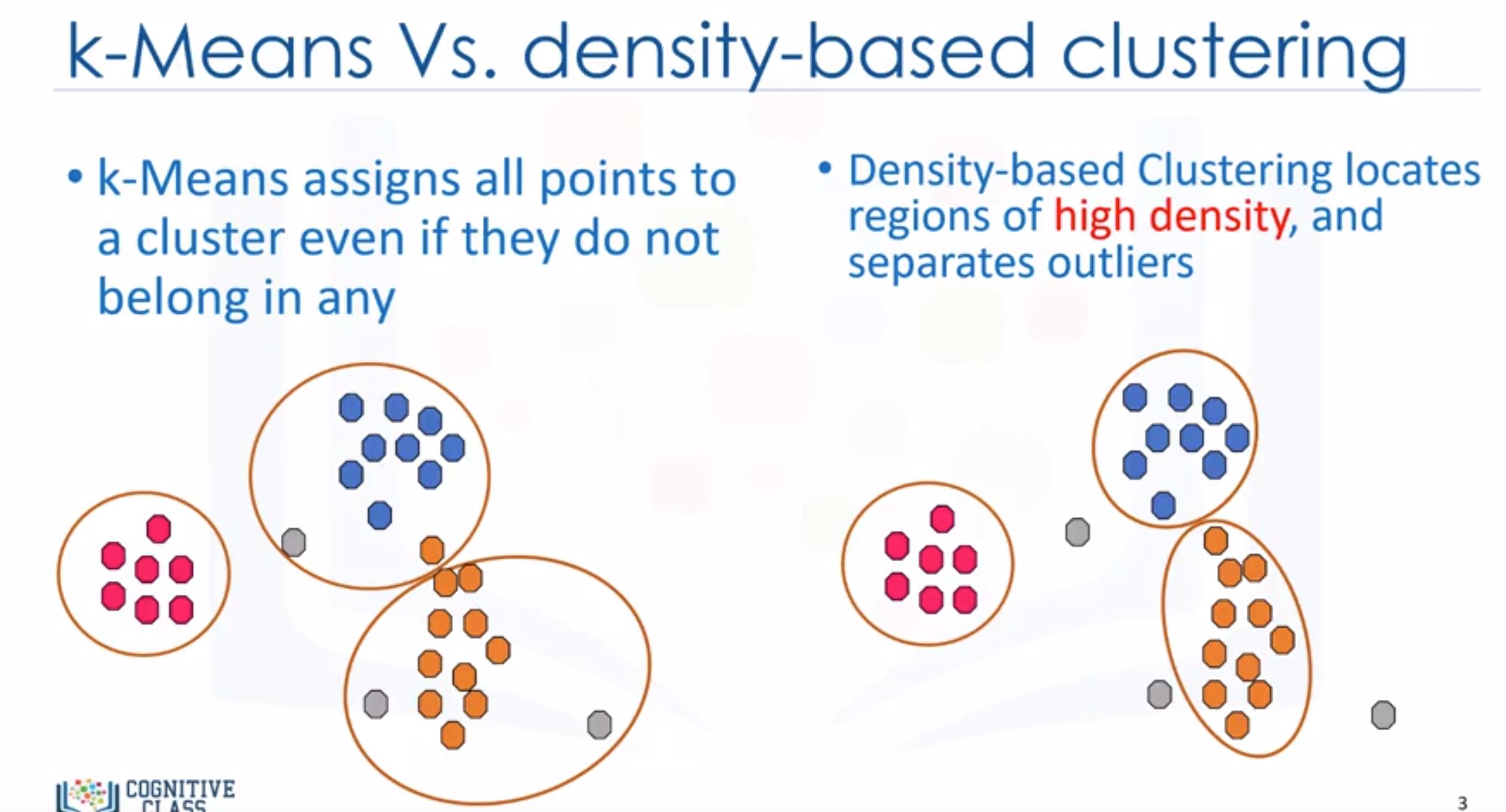
• Density-based clustering locates regions of high density that are separated from one another by regions of low density.
• A specific and very popular type of density-based clustering is DBSCAN (Density-Based Spatial Clustering of Applications with Noise).
  • The wonderful attributes of the DBSCAN algorithm is that it can find out any arbitrary shaped cluster without getting effected by noise.
  • One of the most common clustering algorithm.
  • The algorithm has no notion of outliers that is, all points are assigned to a cluster even if they do not belong in any.
  • Tt does not require one to specify the number of clusters such as K in K-means
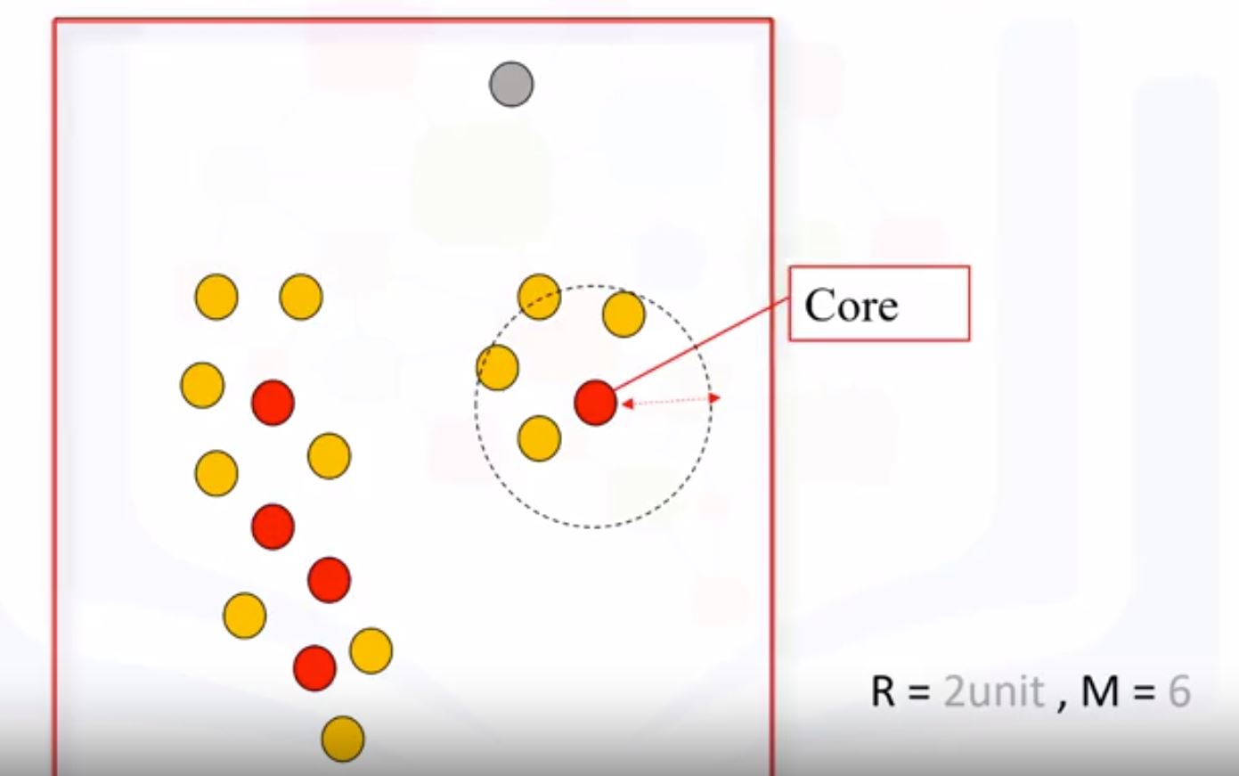
  • 2 parameters
    • R (radius of neighborhood) that if include enough number of points within, we call it a dense area.
    • M (min number of neighbors): the min number of data points we want in a neighborhood to define a cluster.
• DBSCAN ALgorithm: all points fall into 3 types
  • Core point (red) : have enough M points around.
  • Border point (yellow) : in the area of R with other point but have <M points around.
  • Outlier point (gray) : don’t have any points around.

Week 5 : Recommender Systems

Intro to recommender systems

• Recommender systems try to capture these patterns and similar behaviors, to help predict what else you might like.
• There are generally 2 main types of recommendation systems:
  • Content-based : Show me more of the same of what I’ve liked before.
  • Collaborative filtering : Tell me what’s popular among my neighbors, I also may like it.
  • (also) Hybrid recommender systems : combines various mechanisms.
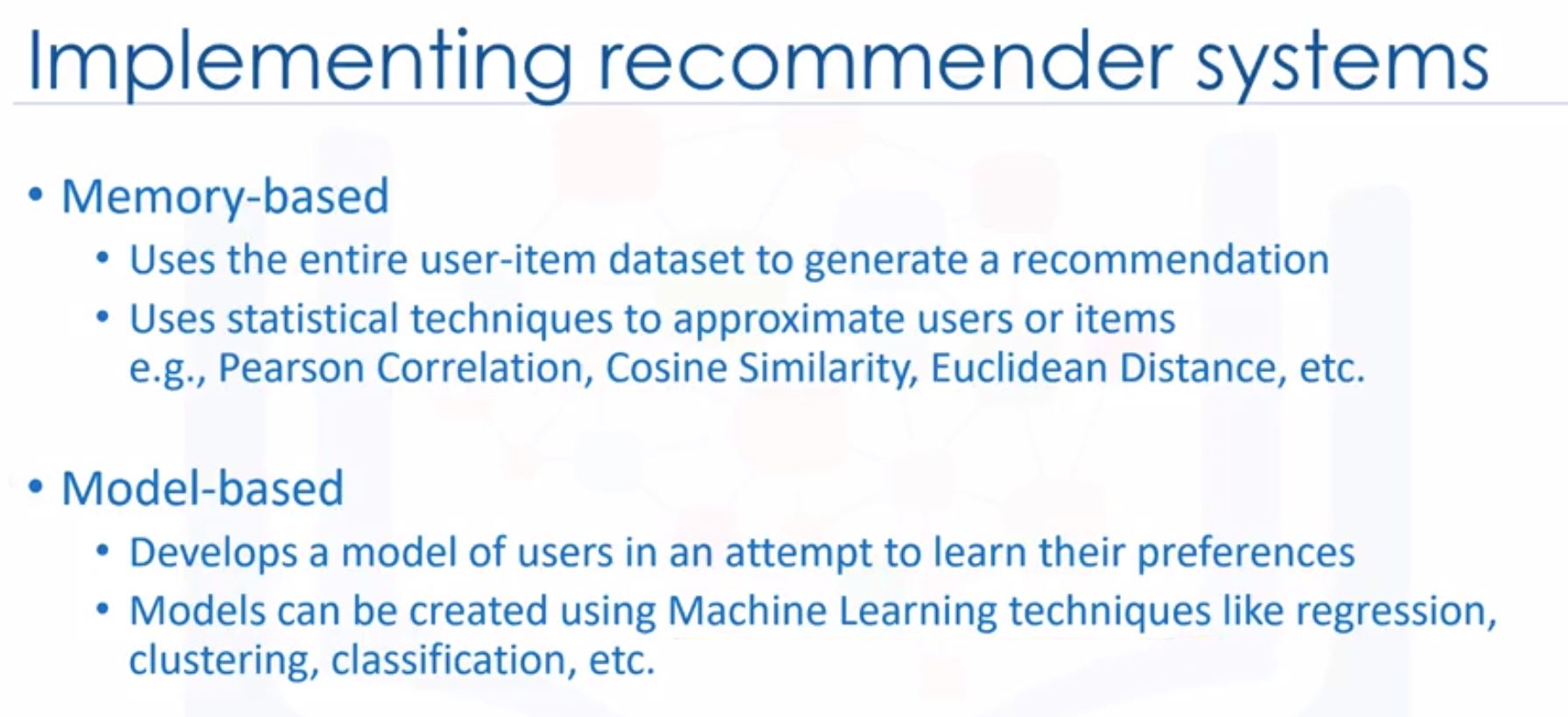
• Implementing recommender systems: Memory-based & Model-based:

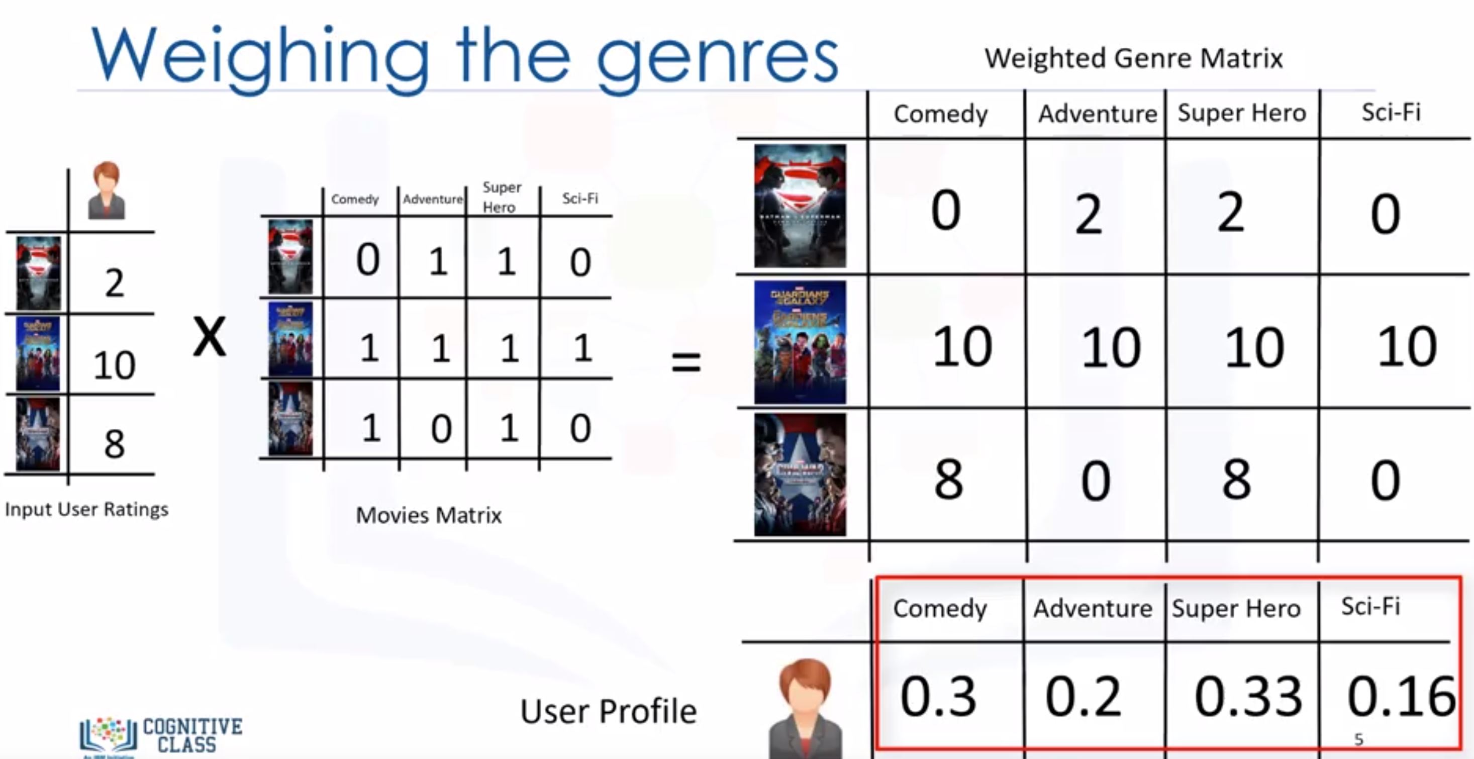
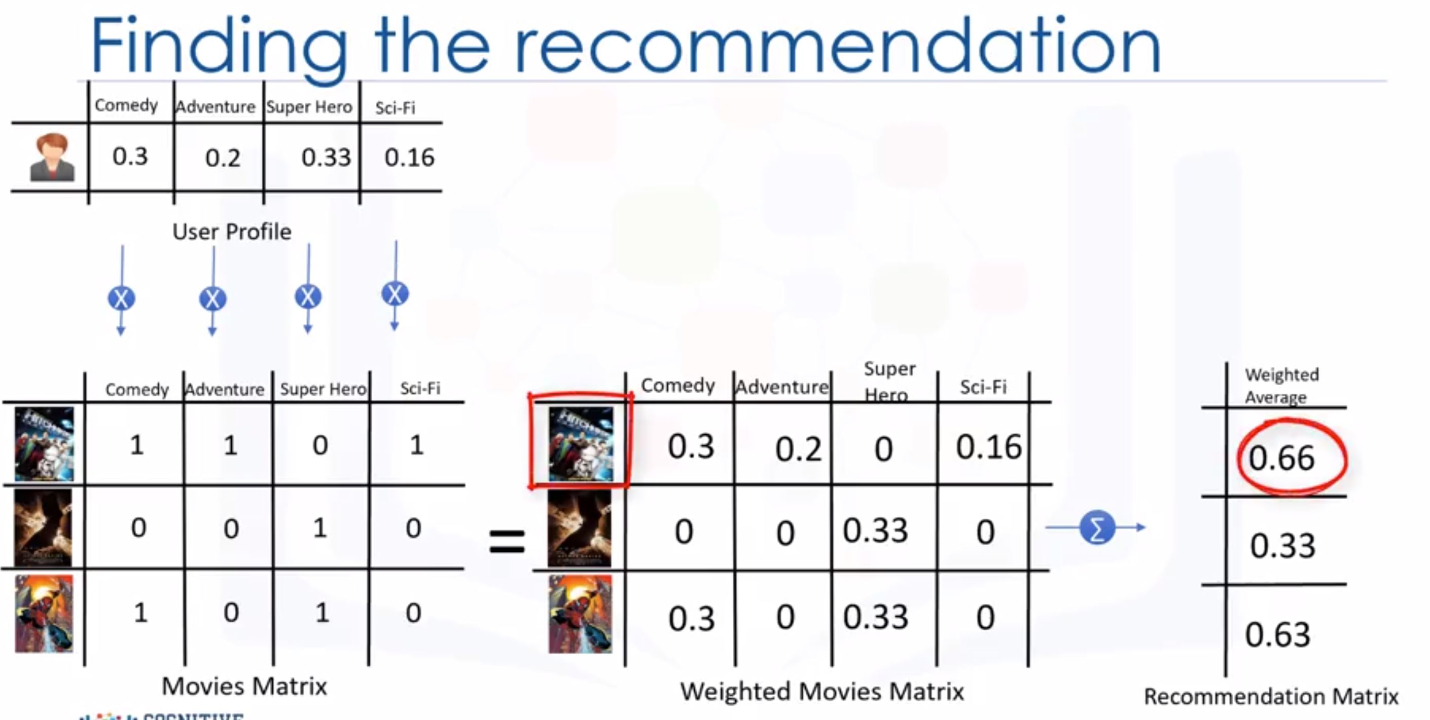
Content-based recommender systems

The lab of Content-based recommender systems

• tries to recommend items to users based on their profile. The user’s profile revolves around that user’s preferences and tastes.
• based on similarity between those items

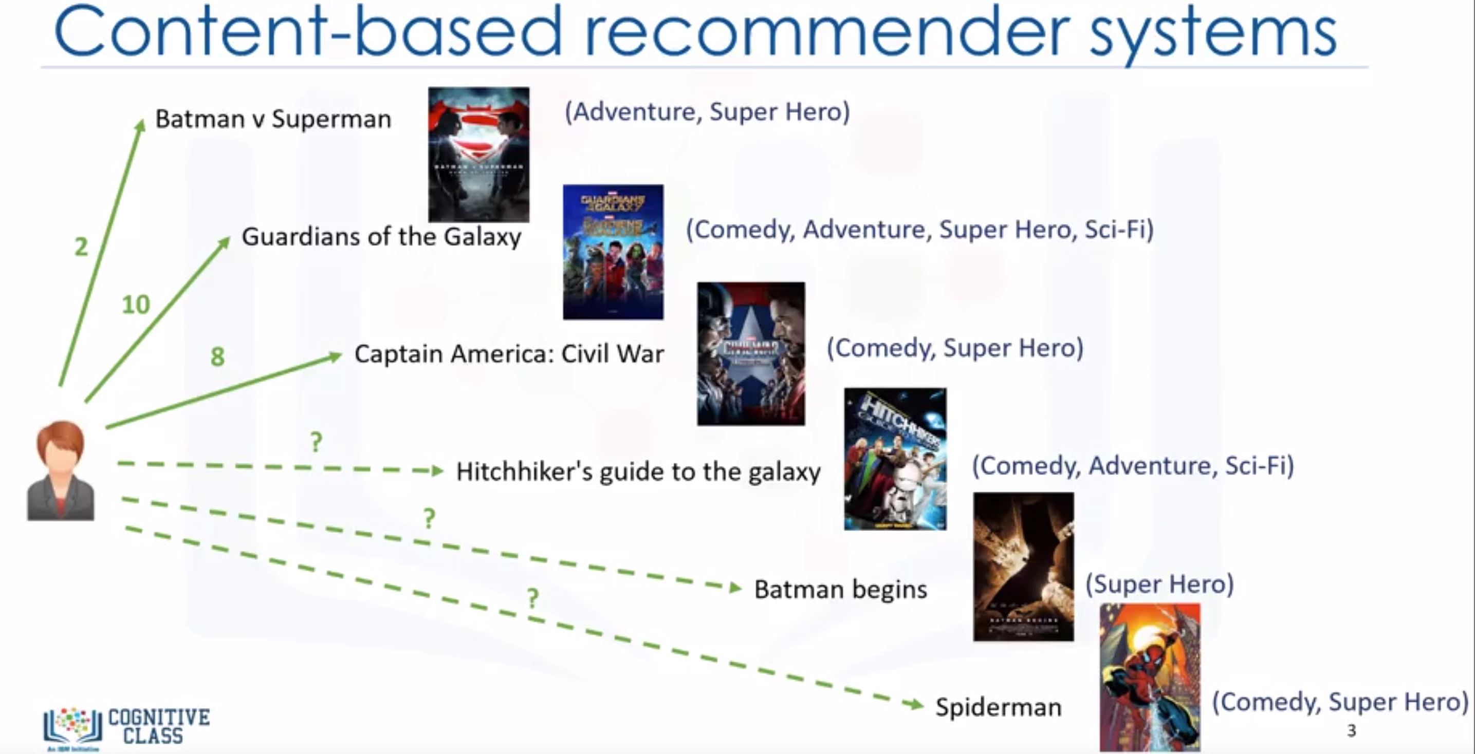
• For a very new genre that the user never watch, the systems didn’t work properly! -> we can use collaborative filering.

Collaborative Filtering

The lab of Collaborative Filtering

• Collaborative filtering is based on the fact that relationships exist between products and people’s interests.
• 2 approaches
  • user-based: based on user’s neighborhood
  • item-based: based on item’s similarity
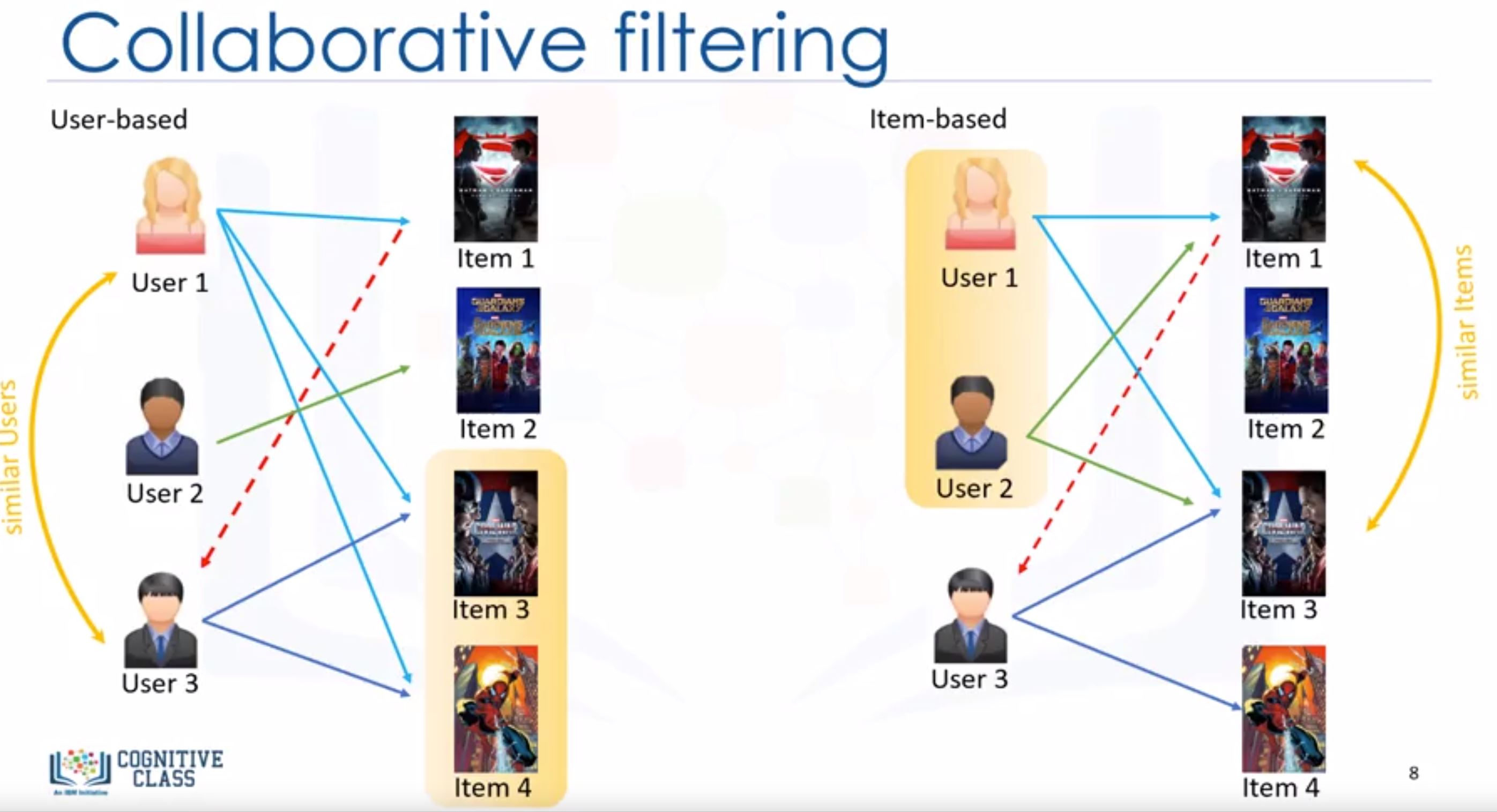
• User-based: if you watch the same movie with your neighbor and she watches a new film, you may like that film too.
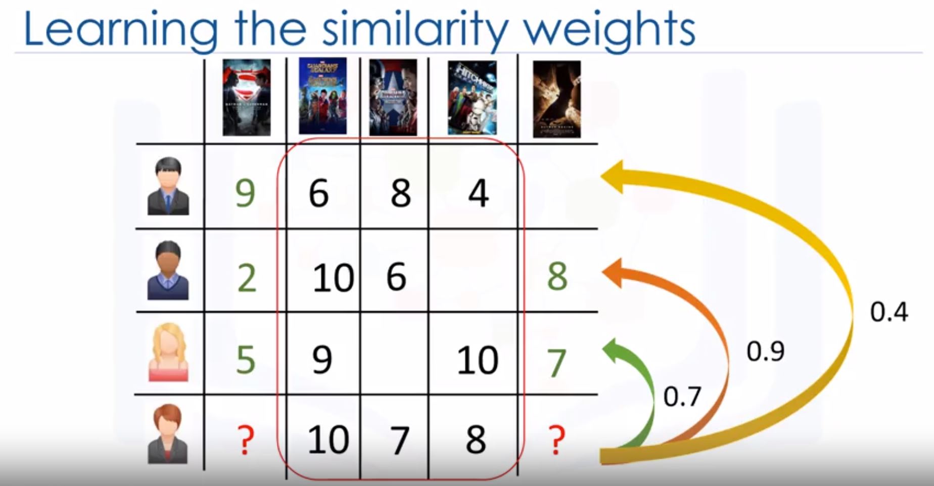
• Find the similar users -> using something like Pearson Correlation Function.
  • Why? Pearson correlation is invariant to scaling, i.e. multiplying all elements by a nonzero constant or adding any constant to all elements. For example, if you have two vectors X and Y,then, pearson(X, Y) == pearson(X, 2 * Y + 3). This is a pretty important property in recommendation systems because for example two users might rate two series of items totally different in terms of absolute rates, but they would be similar users (i.e. with similar ideas) with similar rates in various scales .

• How?

  

  

  

  

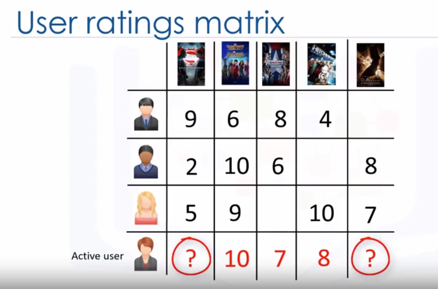
• Process
  • Select a user with the movies the user has watched
  • Based on his rating to movies, find the top X neighbours
  • Get the watched movie record of the user for each neighbour.
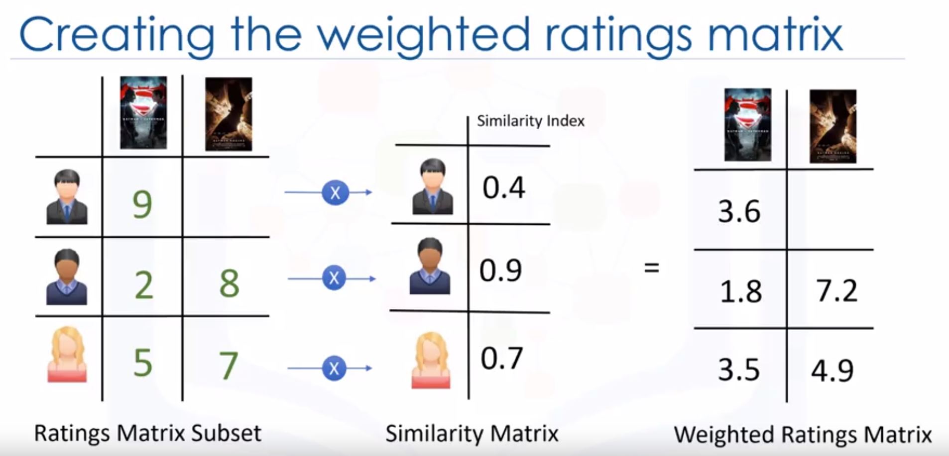
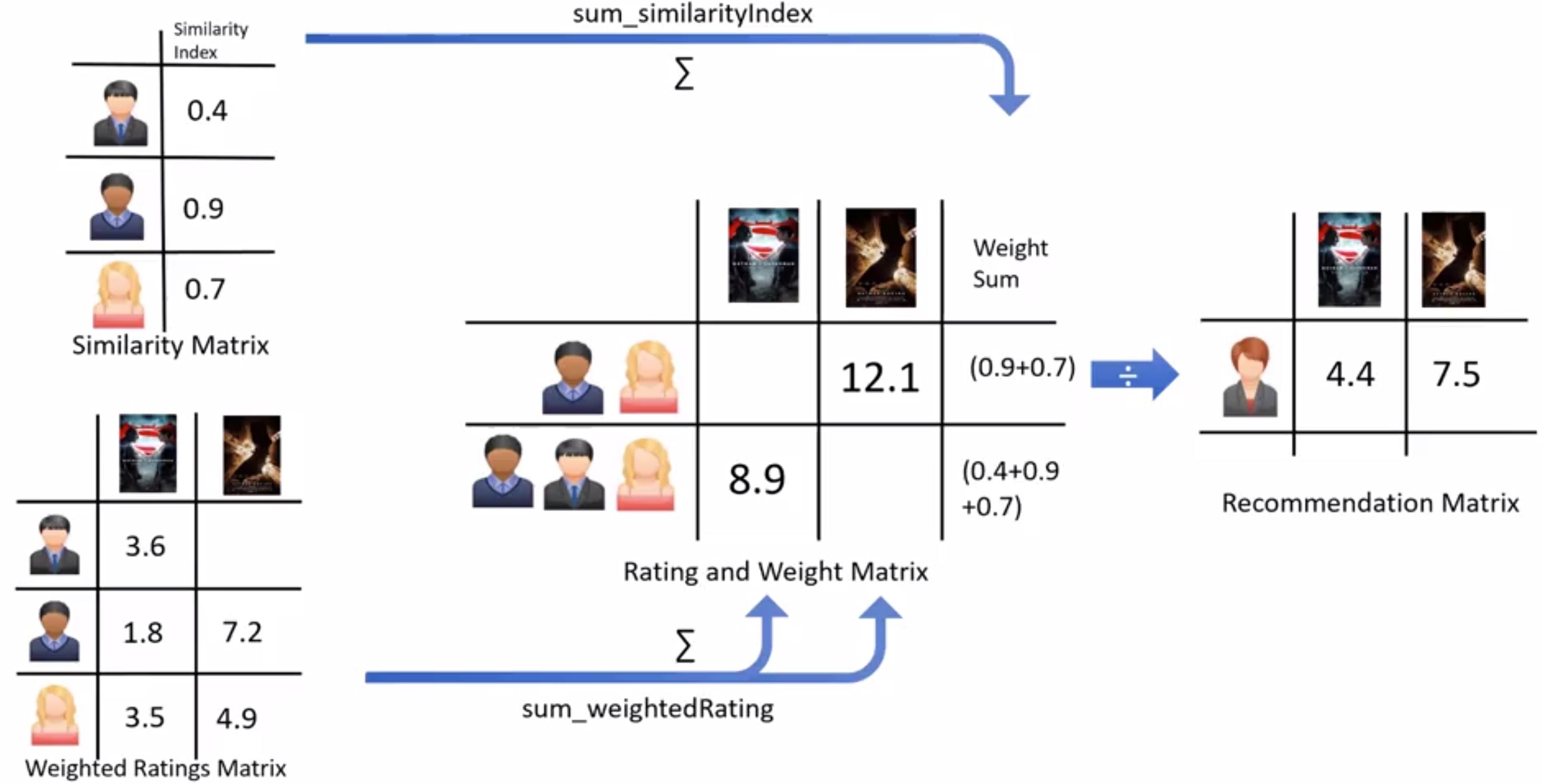
  • Calculate a similarity score using some formula
  • Recommend the items with the highest score
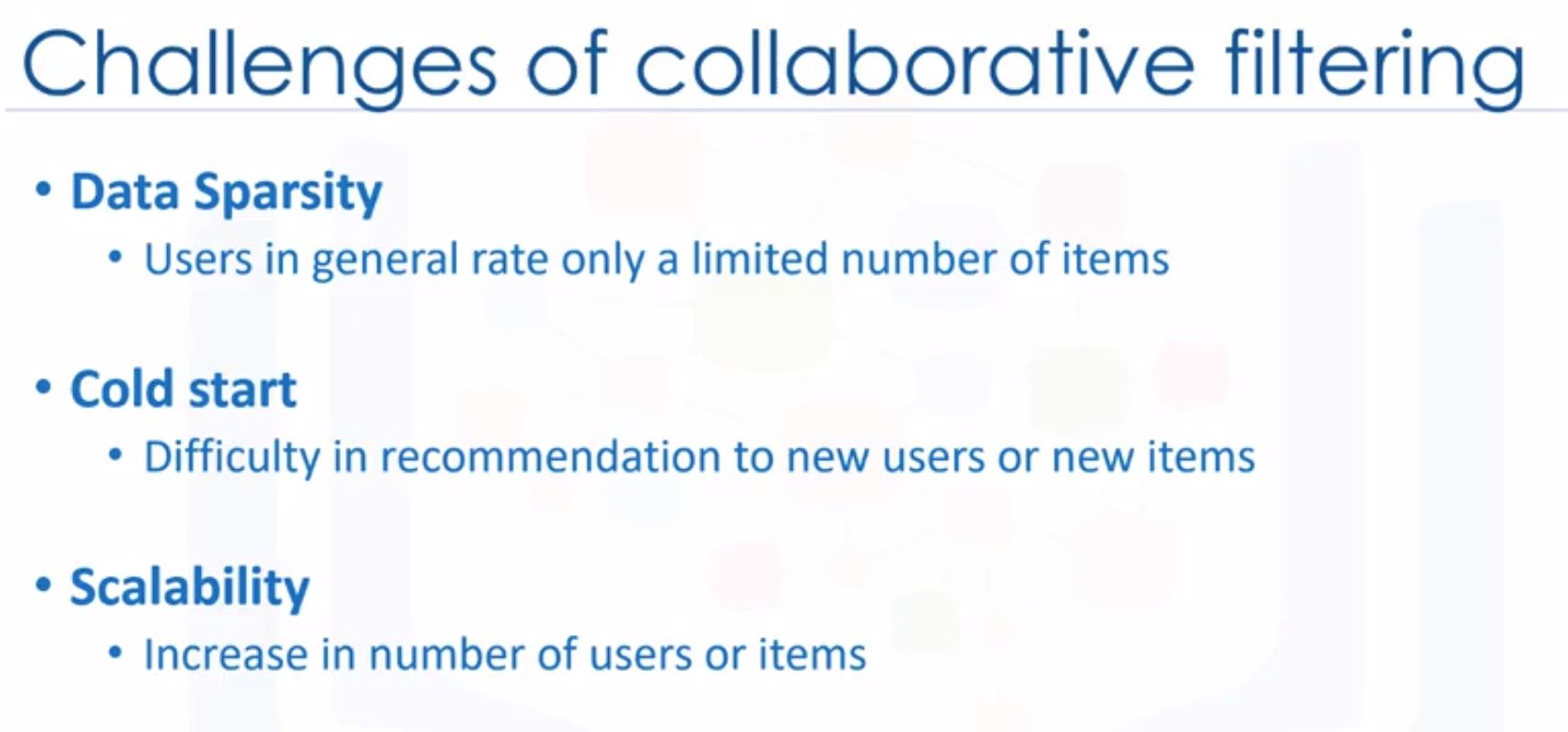
• Challenge of collaborative filtering

Week 6: Final Project

My final project

• You will complete a notebook where you will build a classifier to predict whether a loan case will be paid off or not.
• If you have already sign up and have an account on Watson Studio (previous courses), you can sign in to the page of creating projects here (the guide on the course is not really helpful).