This note was first taken when I learnt the IBM Data Professional Certificate course on Coursera.

Week 1: Introduction to Machine Learning

• What is ML? Machine learning is the subfield of computer science that gives “computers the ability to learn without being explicitly programmed.”
• Major ML techniques:
  • Regression / Estimation: predicting continuous values -> Predicting price of the house based on charateristics
  • Classification: Predicting item class/category of a case -> If a cell is benign or malignant
  • Clustering: Finding the structure of data / summarization -> can find similar patients, or can be used for customer segmentation in the banking field.
  • Association: Associating frequent co-occuring items/events -> grocery items that are usually bought together by a particular customer.
  • Anomaly detection: Discovering abnormal and unusual cases -> it is used for credit card fraud detection.
  • Sequence mining: Predicting next events, click-stream (Markov Model, HMM) -> the click-stream in websites.
  • Dimension Reduction: Reducing the size of data (PCA)
  • Recommendation systems: Recommending items -> associates people’s preferences with others who have similar tastes, and recommends new items to them, such as books or movies.
• ML vs AI vs Deep Learning:
  • AI: make computer smarter like a human (computer vision, language processing, creativity,…)
  • ML: a branch of AI. It teaches computer to solve problems, learning from thousands of examples to solve the same problem in new situations.
  • Deep Learning: a special case of ML where computer learn and make intelligent decisions on their own.
• Python for ML:
  • numpy: is a math library to work with N-dimensional arrays in Python. It enables you to do computation efficiently and effectively.
  • scipy: is a collection of numerical algorithms and domain specific toolboxes, including signal processing, optimization, statistics and much more. SciPy is a good library for scientific and high performance computation.
  • Matplotlib: provides 2D plotting, as well as 3D plotting.
  • Pandas: provides high performance easy to use data structures. It has many functions for data importing, manipulation and analysis. In particular, it offers data structures and operations for manipulating numerical tables and timeseries.
  • scikitlearn: a collection of algorithms and tools for machine learning.
    • It has most of the classification, regression and clustering algorithms, and it’s designed to work with a Python numerical and scientific libraries; NumPy and SciPy.
    • Most of the tasks that need to be done in a machine learning pipeline are implemented already in Scikit Learn including pre-processing of data, feature selection, feature extraction, train test splitting, defining the algorithms, fitting models, tuning parameters, prediction, evaluation and exporting the model.
• Supervised vs Unsupervised
  • Supervsised learning: means to observe, and direct the execution of a task, project, or activity.
    • We teach the model by training it with some data from a labeled dataset.
    • 2 types: classification vs regression
    • deal with labeled data
  • unsupervised learning: is exactly as it sounds. We do not supervise the model, but we let the model work on its own to discover information that may not be visible to the human eye.
    • unsupervised learning has more difficult algorithms than supervised learning since we know little to no information about the data, or the outcomes that are to be expected.
    • clustering
    • deal with unlabeled data

Week 2: Regression

info - Check the lab: simple linear regression for the example and guide. - the lab: multiple linear regression - the lab: polynomial regression - - the lab: non-linear regression

Linear regression

• The key point in the regression, is that our dependent value should be continuous, and cannot be a discrete value. -> quantity
• 2 types of regressions:
  • simple regression: linear/non-linear regression
  • multiple regression: multiple linear/non-linear regression
• Examples:
  • Sales forecasting
  • Sastisfaction analysis
  • Price estimation
  • Employment income
• Algorithms
  • Ordinal regression
  • Poisson regression
  • Fast forest quantile regression
  • Linear, Polynomial, Lasso, Stepwise, Ridge regression
  • Bayesian network regression
  • Decision forest regression
  • Boosted decision tree regression
  • KNN (K-nearest neighbors)
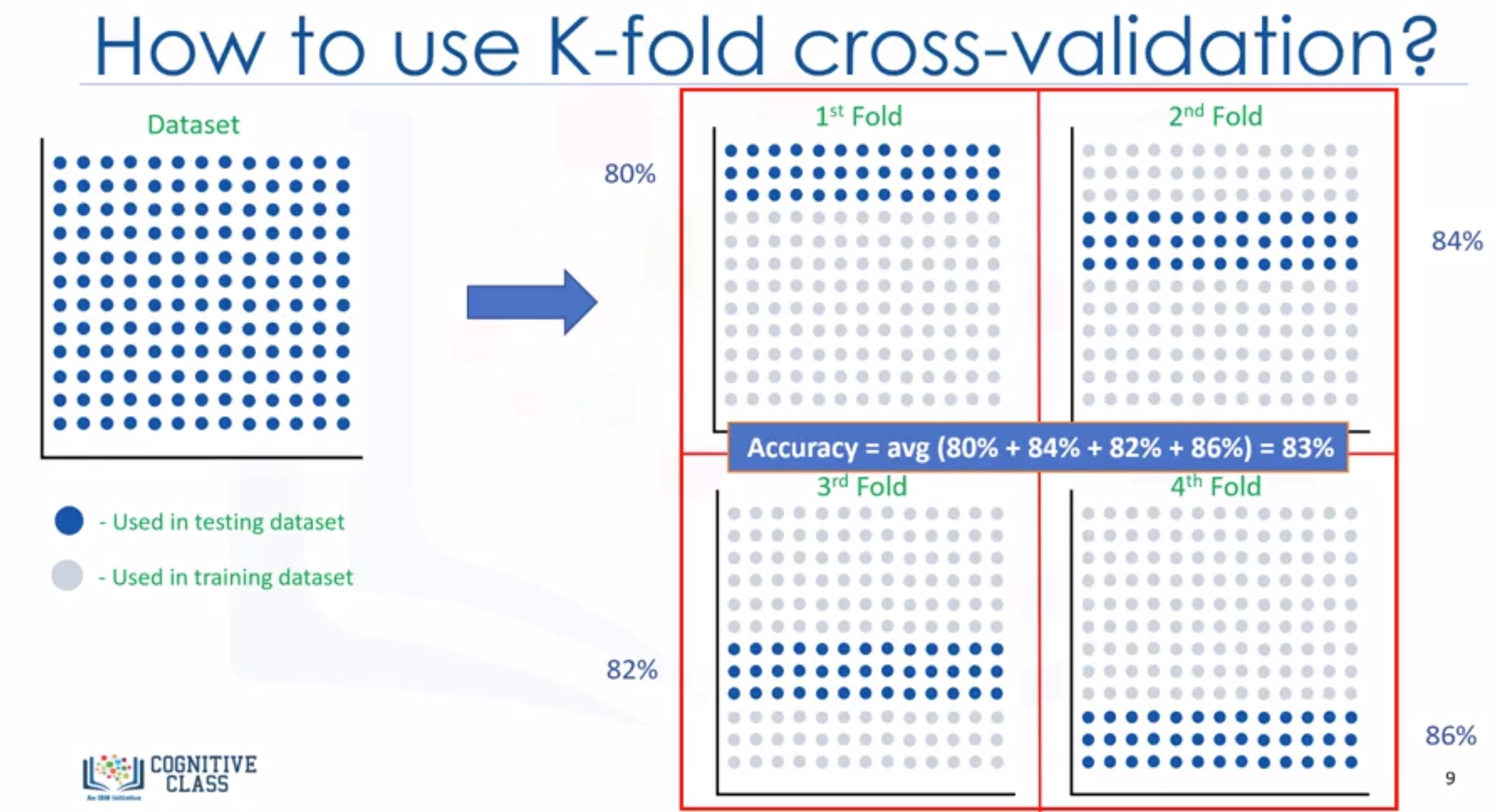
• Training accuracy: is the percentage of correct predictions that the model makes when using the test dataset.
  • High training accuracy is not a good thing -> may overfitting!
• Out-of-sample accuracy is the percentage of correct predictions that the model makes on data that the model has not been trained on.
  • It’s important that our models have high out-of-sample accuracy
  • Highly dependent on which dataset the data is trained and tested.
• K-fold cross-validation: K-fold cross-validation in its simplest form performs multiple train/test splits, using the same dataset where each split is different.
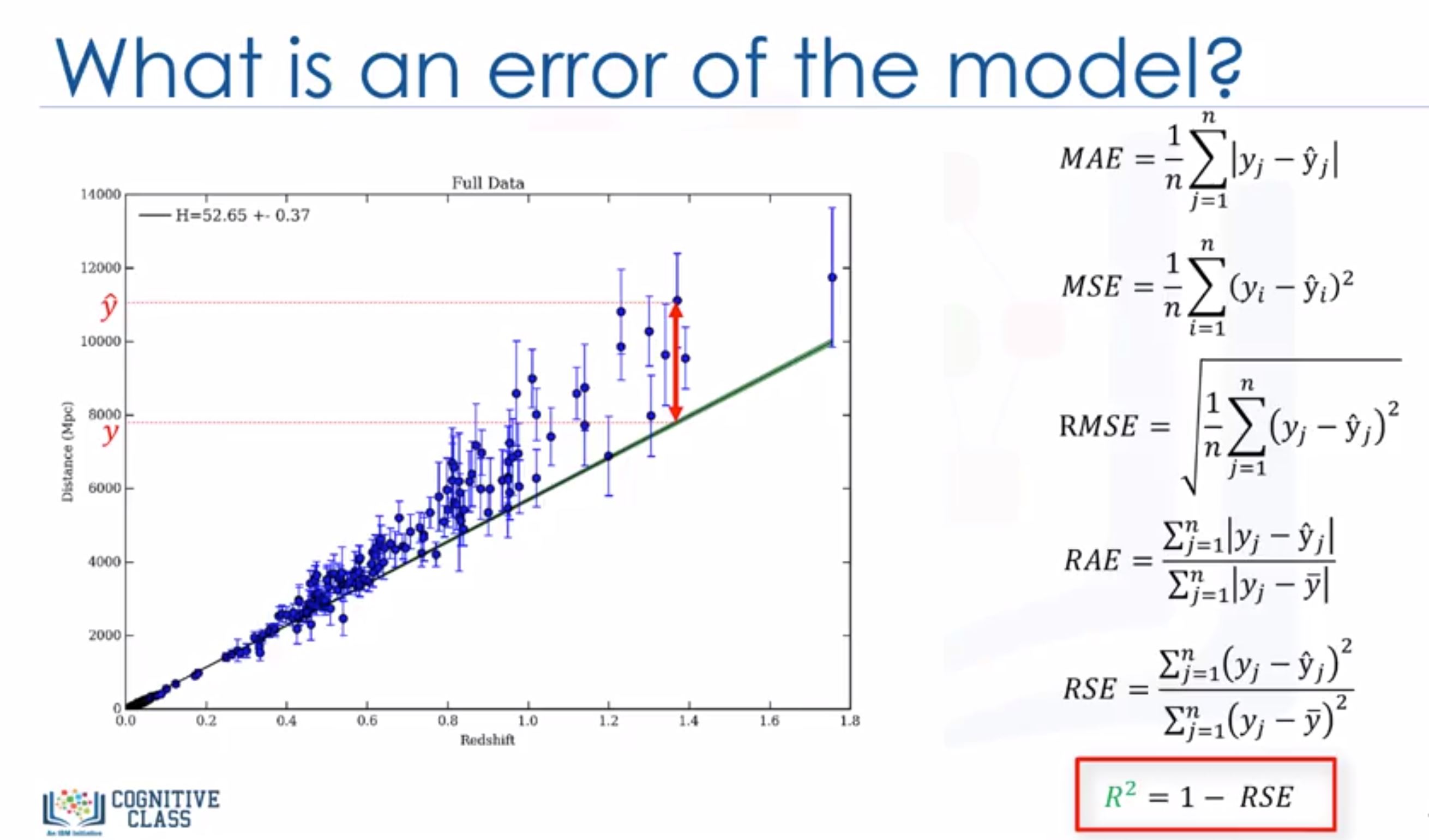
• Errors metrics: the higher $R^2$, the better your model fit your data.
• Multiple regression
  • First, it can be used when we would like to identify the strength of the effect that the independent variables have on the dependent variable.
  • Second, it can be used to predict the impact of changes, that is, to understand how the dependent variable changes when we change the independent variables.
  • Using many variables -> overfitting
  • Using scatter plot to check if there is a linear regression. If not, use non-linear regression.
• Ordinary Least Squares (OLS): OLS is a method for estimating the unknown parameters in a linear regression model. OLS chooses the parameters of a linear function of a set of explanatory variables by minimizing the sum of the squares of the differences between the target dependent variable and those predicted by the linear function. In other words, it tries to minimizes the sum of squared errors (SSE) or mean squared error (MSE) between the target variable (y) and our predicted output ($\hat{y}$) over all samples in the dataset.
  • Solving the model parameters analytically using closed-form equations
  • Using an optimization algorithm (Gradient Descent, Stochastic Gradient Descent, Newton’s Method, etc.)

Non-linear regression

• What: First, non-linear regression is a method to model a non-linear relationship between the dependent variable and a set of independent variables. Second, for a model to be considered non-linear, Y hat must be a non-linear function of the parameters Theta, *not necessarily the features *X. $\hat{y} = \theta_0 + \theta_1\theta_2^x$
• Polynomial regression:
  • Polynomial regression fits a curve line to your data.
  • a polynomial regression model can still be expressed as linear regression.
  • Therefore, polynomial regression models can fit using the model of least squares. Least squares is a method for estimating the unknown parameters in a linear regression model by minimizing the sum of the squares of the differences between the observed dependent variable in the given dataset and those predicted by the linear function.

Week 3: Classification

info Labs - KNN - Decision Trees

• Classification
  • Supervised learning approaches.
  • We can also build classifier models for both binary classification and multi-class classification.
• Multiclass classifier: A classifier that can predict a field with multiple discrete values, such as “DrugA”, “DrugX” or “DrugY”.
• For example, classification can be used for email filtering, speech recognition, handwriting recognition, biometric identification, document classification and much more.
• Classification algorithms in machine learning:
  • decision trees,
  • naive bayes,
  • linear discriminant analysis,
  • k-nearest neighbor,
  • logistic regression,
  • neural networks,
  • support vector machines.

K-nearest Neighbours

• This is a classification algorithm, we choose a categories for some example based on the category of their neighbors. For example, if $K=1$, the category of that example is the same with the category of the nearest example to it.
• Calculate the accuracy with different numbers of $K$ and then choose the best one.

Evaluation Metrics in Classification

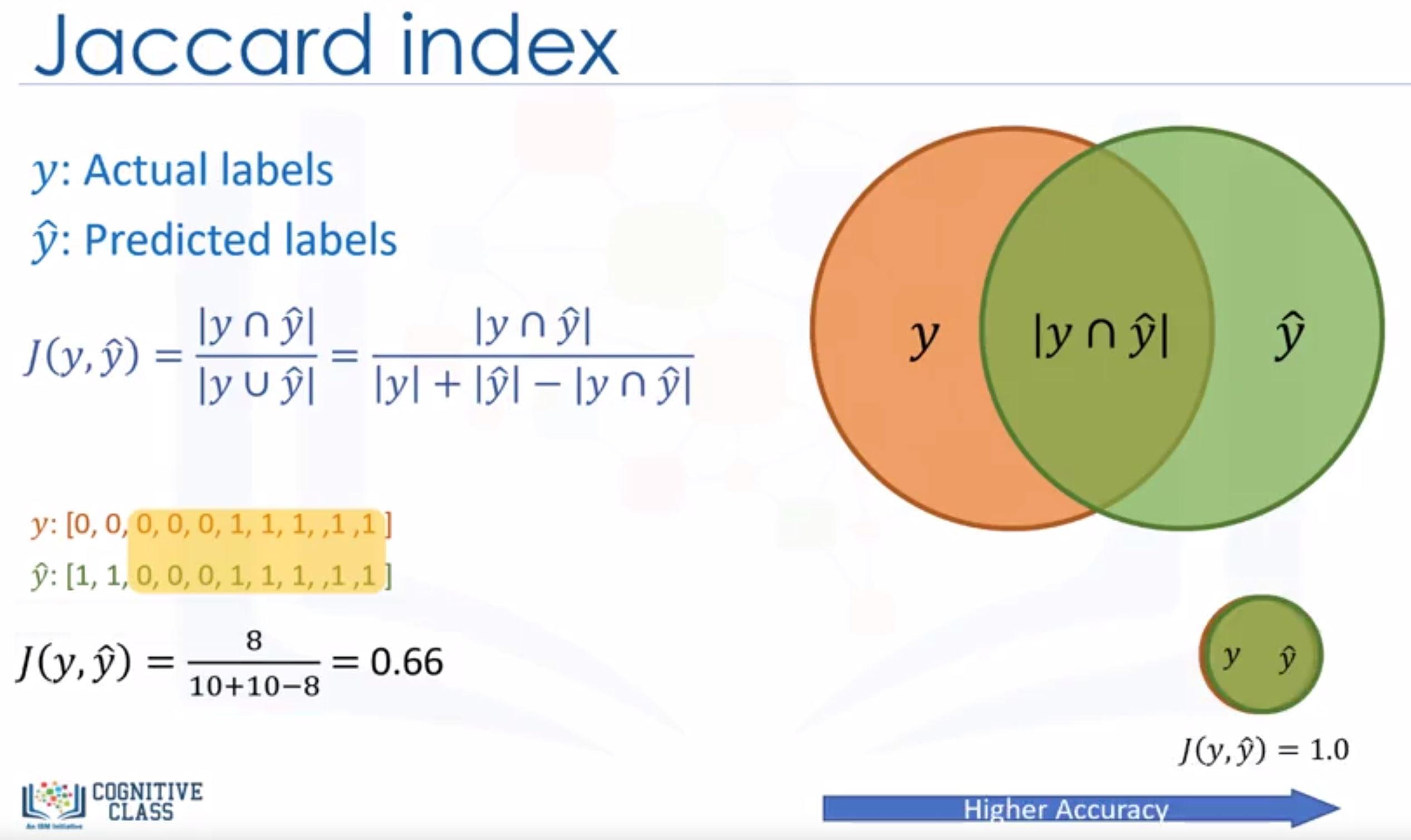
• Jaccard index: higher is better
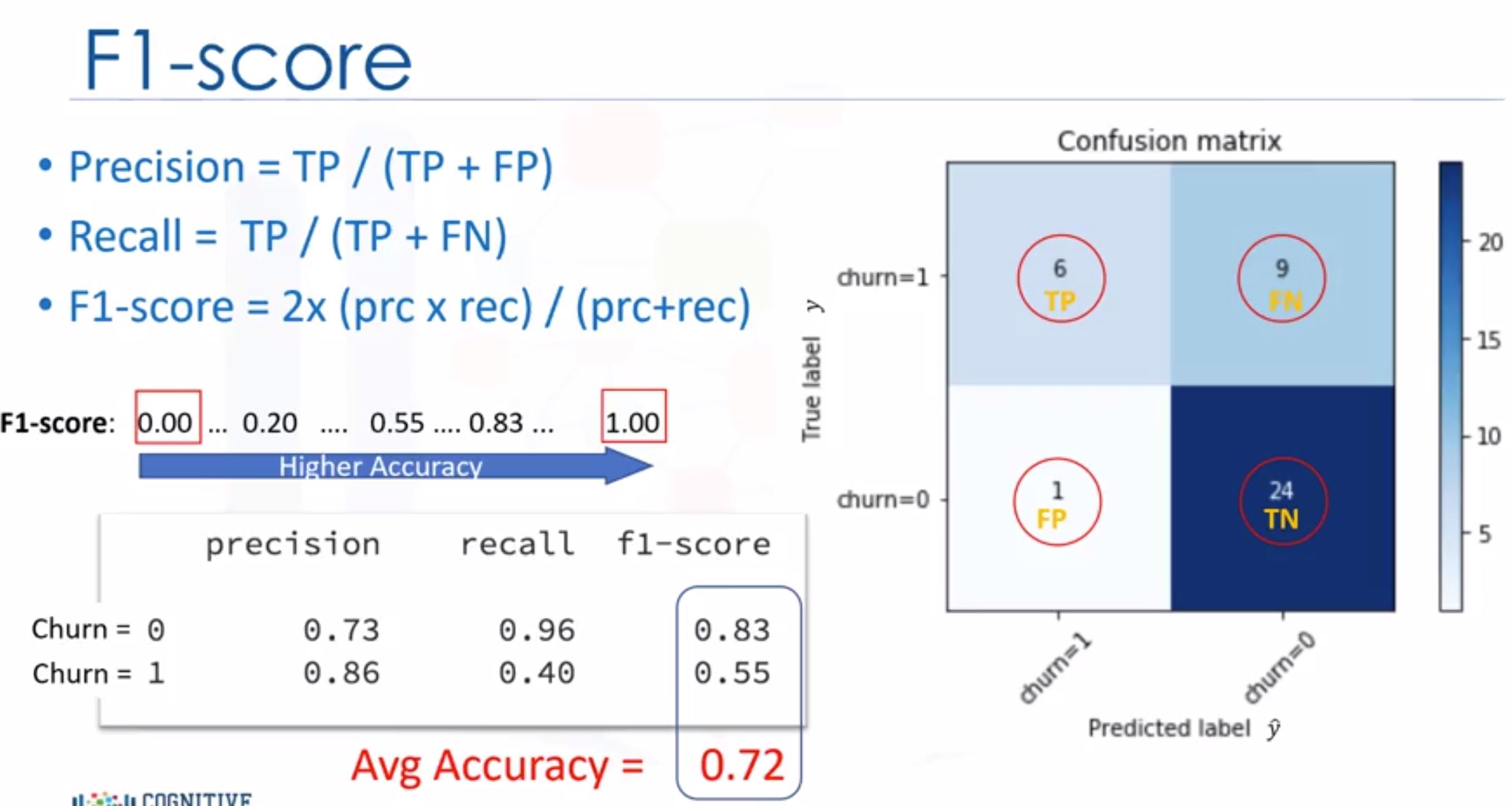
• F1-Score: higher is better
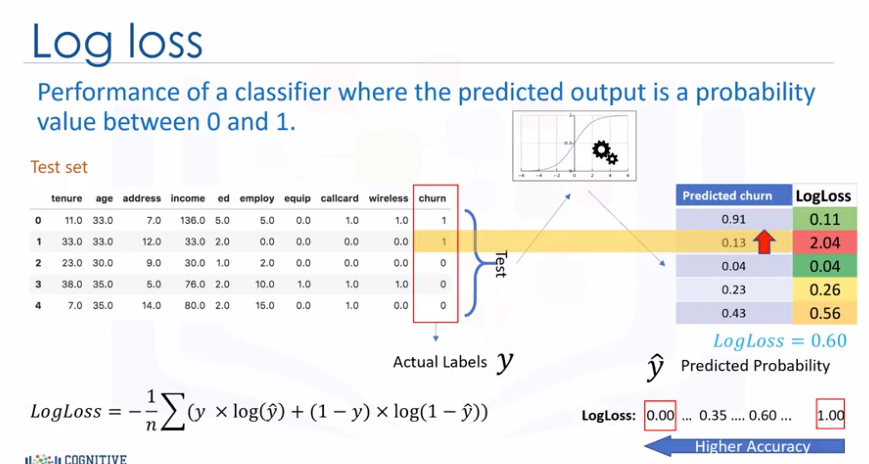
• Log Loss: Logarithmic loss (also known as Log loss) measures the performance of a classifier where the predicted output is a probability value between 0 and 1. We can calculate the log loss for each row using the log loss equation, which measures how far each prediction is, from the actual label.

From the labs

Load data file and show the 1st 5 lines

df = pd.read_csv('teleCust1000t.csv')
df.head()

See how many of each class in your data set

df['custcat'].value_counts()

Visualize your income colum in histogram

df.hist(column='income', bins=50)

List all of columns’ name in your data set

df.hist(column='income', bins=50)

To use scikit-learn library, we have to convert the Pandas data frame to a Numpy array:

X = df[['col1', 'col2', 'col3']].values

Check the values of some column

df['custcat'].values

Normalize data (zero mean, unit variance,…)

from sklearn import preprocessing
X = preprocessing.StandardScaler().fit(X).transform(X.astype(float))

Split the data into training/test sets

from sklearn.model_selection import train_test_split
X_train, X_test, y_train, y_test = train_test_split( X, y, test_size=0.2, random_state=4)

Using K-nearest neighbor (KNN)

from sklearn.neighbors import KNeighborsClassifier
k = 4
#Train Model and Predict  
neigh = KNeighborsClassifier(n_neighbors = k).fit(X_train,y_train)
yhat = neigh.predict(X_test)

Accuracy evaluation

from sklearn import metrics
print("Train set Accuracy: ", metrics.accuracy_score(y_train, neigh.predict(X_train)))
print("Test set Accuracy: ", metrics.accuracy_score(y_test, yhat))

Decision tree

• The basic intuition behind a decision tree is to map out all possible decision paths in the form of a tree.
• Decision tree learning algorithm
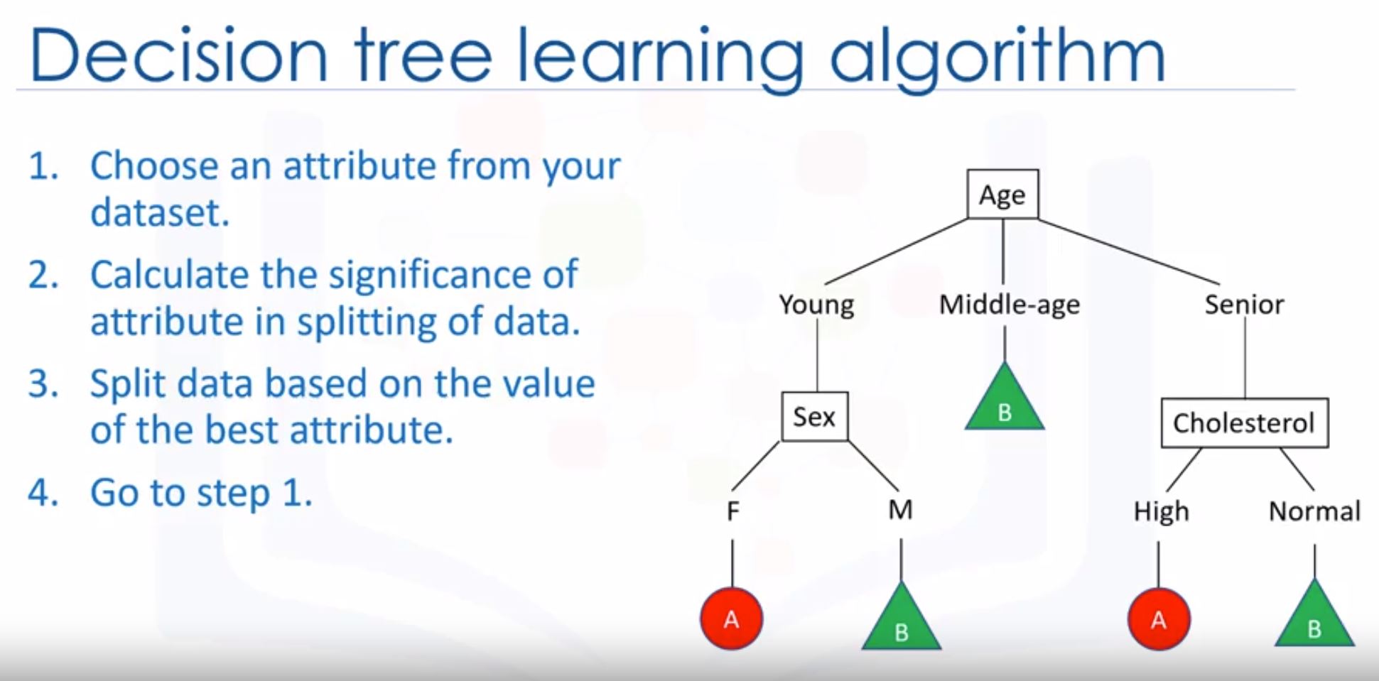
• What is important in making a decision tree, is to determine which attribute is the best or more predictive to split data based on the feature.
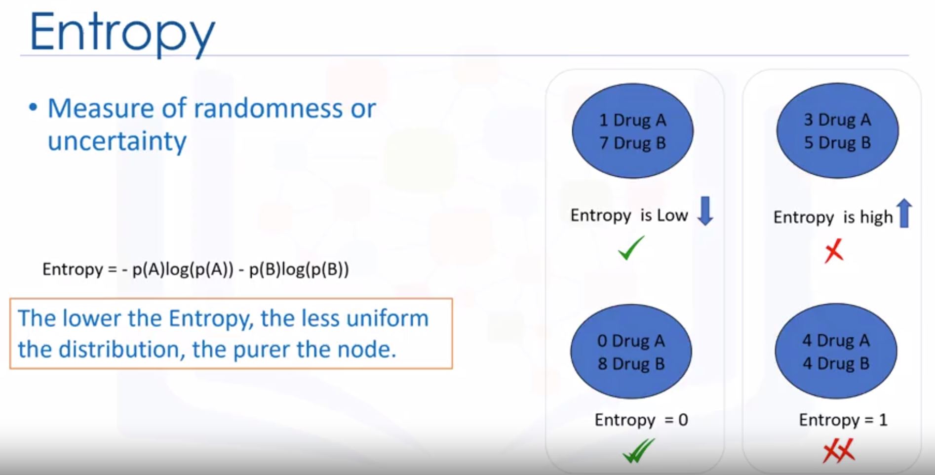
• Entropy is the amount of information disorder or the amount of randomness in the data.
  • The lower the entropy, the less uniform the distribution, the purer the node.
  • How we decide which entropy is better? -> the tree with the higher information gain after splitting.

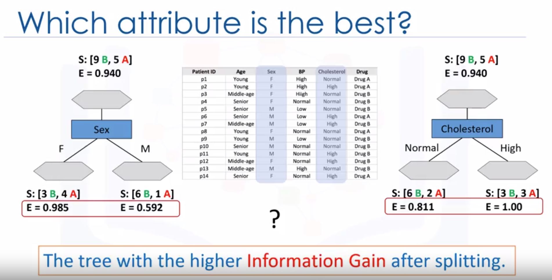
  • information gain: is the information that can increase the level of certainty after splitting.

    $$\text{information gain} = \text{entropy before split} - \text{weighted entropy after split}$$
  • Bigger information gain, smaller entropy -> choose the tree with smaller entropy value.
• Sklearn Decision Trees do not handle categorical variables.
  • We can convert these features to numerical values using pandas.get_dummies()

From the lab

Libraries for the decision tree

import numpy as np 
import pandas as pd
from sklearn.tree import DecisionTreeClassifier

The size of data

my_data = pd.read_csv("drug200.csv", delimiter=",")
my_data.shape

Convert categorical variable into dummy/indicator variables (category to numeric)

le_BP = preprocessing.LabelEncoder()
le_BP.fit([ 'LOW', 'NORMAL', 'HIGH'])
X[:,2] = le_BP.transform(X[:,2])

Setting up the decision tree

X_trainset, X_testset, y_trainset, y_testset = train_test_split(X, y, test_size=0.3, random_state=3)
drugTree = DecisionTreeClassifier(criterion="entropy", max_depth = 4)
# train
drugTree.fit(X_trainset,y_trainset)
# predict
predTree = drugTree.predict(X_testset

Evaluation metrics for decision tree

from sklearn import metrics
print("DecisionTrees's Accuracy: ", metrics.accuracy_score(y_testset, predTree))

# calculate the accuracy score without sklearn
np.mean(predTree==y_testset)

Visualization decision tree

# Notice: You might need to uncomment and install the pydotplus and graphviz libraries if you have not installed these before
# !conda install -c conda-forge pydotplus -y
# !conda install -c conda-forge python-graphviz -y

from sklearn.externals.six import StringIO
import pydotplus
import matplotlib.image as mpimg
from sklearn import tree

dot_data = StringIO()
filename = "drugtree.png"
featureNames = my_data.columns[0:5]
targetNames = my_data["Drug"].unique().tolist()
out=tree.export_graphviz(drugTree,feature_names=featureNames, out_file=dot_data, class_names= np.unique(y_trainset), filled=True,  special_characters=True,rotate=False)  
graph = pydotplus.graph_from_dot_data(dot_data.getvalue())  
graph.write_png(filename)
img = mpimg.imread(filename)
plt.figure(figsize=(100, 200))
plt.imshow(img,interpolation='nearest')
# plt.show()

Logistic regresstion

info - Check the lab: logistic regression.

• LR is a classification algorithm for categorical variables.
• Logistic regression is analogous to linear regression, but tries to predict a categorical or discrete target field instead of a numeric one.
• Can be used for binary classification and multiclass classification.
• Examples to be applied LR
  • Predicting the probability of a person having a heart attack
  • Predicting the mortality in injured patients
  • Predicting a customer’s propensity to purchase a product or halt a subsription
  • Predicting the probability of failure of a given process or product
  • Predicting the likelihood of a homeowner defaulting on a mortage
• When is logistic regression suitable?
  • If your data is binary (0/1, yes/no, positive/negative)
  • If you need probabilities results.
  • When you need a linear decision boundary
  • If you need to understand the impact of feature.
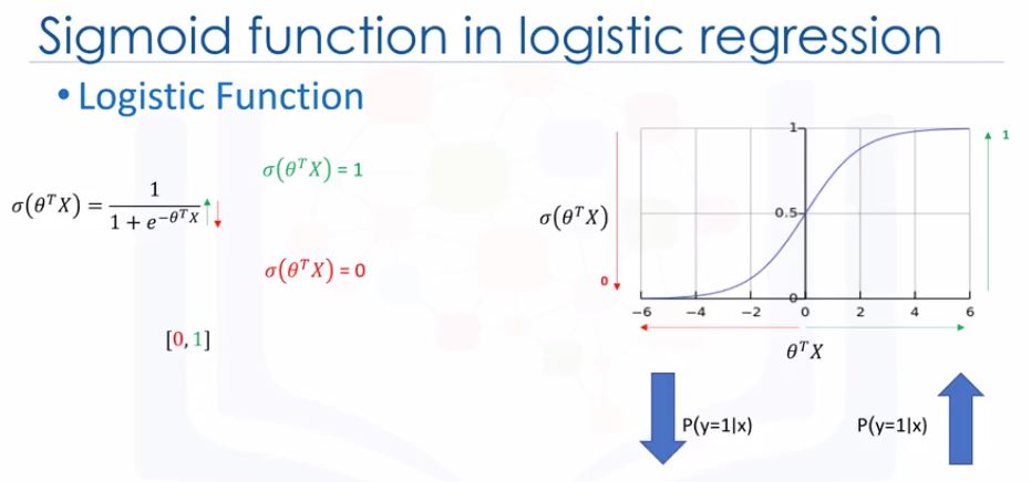
• Sigmoid function (logistic function): $\sigma(\theta^TX) = \dfrac{1}{1+e^{-\theta^TX}}$
  • always between 0 and 1
  • The training process
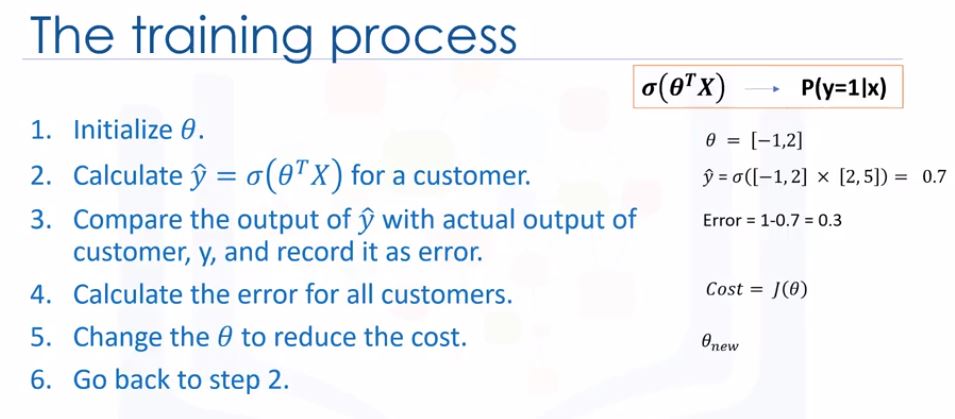
  • Change the values of $\theta$ using gradient descent
  • When should we stop the iteration? -> calculating the accuracy of your model and stop it when it’s satisfactory. $J(\theta) = -\frac{1}{m} \sum_{i=1}^m y^i \log(\hat{y}^i) + (1-y^i)\log(1-\hat{y}^i)$
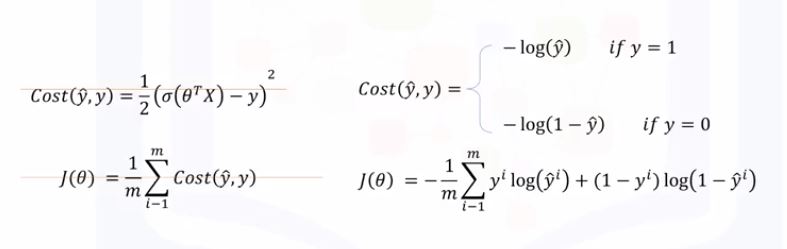
• Minimize the cost function of the model
  • optimization approach: gradient descent: use derivative of cost function to change values of the parameters

The lab of logistic regression

Link to ref

Convert all values to int type

churn_df['churn'] = churn_df['churn'].astype('int')

Get the name of columns

churn_df.columns.values

Defin X, y as adday in numpy

X = np.asarray(churn_df[['tenure', 'age', 'address', 'income', 'ed', 'employ', 'equip']])
y = np.asarray(churn_df['churn'])

Normalize the dataset

from sklearn import preprocessing
X = preprocessing.StandardScaler().fit(X).transform(X)

Train/test dataset

from sklearn.model_selection import train_test_split
X_train, X_test, y_train, y_test = train_test_split( X, y, test_size=0.2, random_state=4)

Logistic regression with scikit-learn (support regularization which is a technique used to solve the overfitting problem in machine learning models)

from sklearn.linear_model import LogisticRegression
LR = LogisticRegression(C=0.01, solver='liblinear').fit(X_train,y_train)
# C parameter indicates inverse of regularization strength which must be a positive float.
yhat = LR.predict(X_test)

# get the probability
#  the first column is the probability of class 1, P(Y=1|X), and second column is probability of class 0, P(Y=0|X):
yhat_prob = LR.predict_proba(X_test)

Evaluations

# jaccard index
from sklearn.metrics import jaccard_similarity_score
jaccard_similarity_score(y_test, yhat)

# confusion matrix -> check the lab for more
from sklearn.metrics import classification_report
classification_report(y_test, yhat)

# log loss
from sklearn.metrics import log_loss
log_loss(y_test, yhat_prob)

Support Vector Machine (SVM)

info - Check the lab: SVM.

• used for classification
• SVM = a supervised algorithm that classifies cases by finding a separator.
  1. Mapping data to a higher-dimensional feature space
  2. Finding a separator
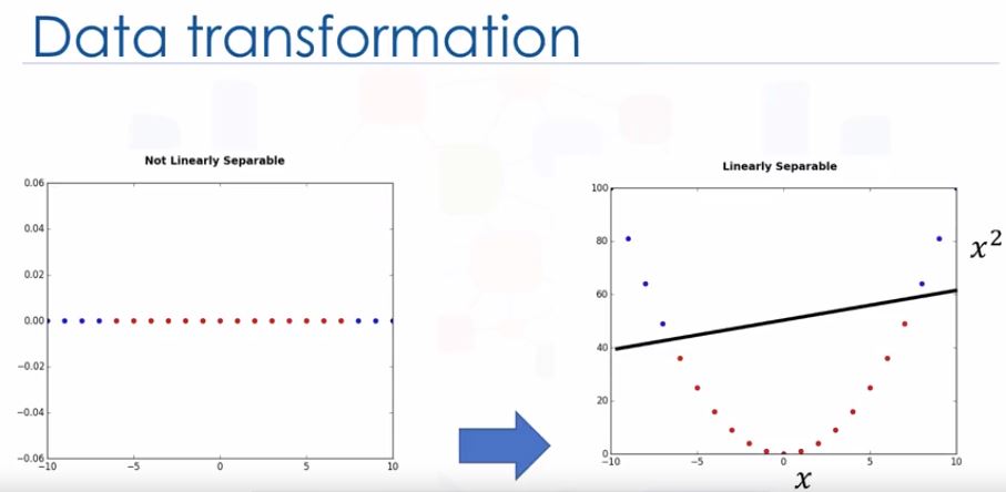
• Sometimes, the line between 2 features are complicated curves, that means it’s difficult to find. However, after transform the problem to higher dimension, we can separated the features by a plane, for example, it’s clearer.
  • 1st question: how do we transfer data in such a way a separator could be draw as a plane? -> kernelling
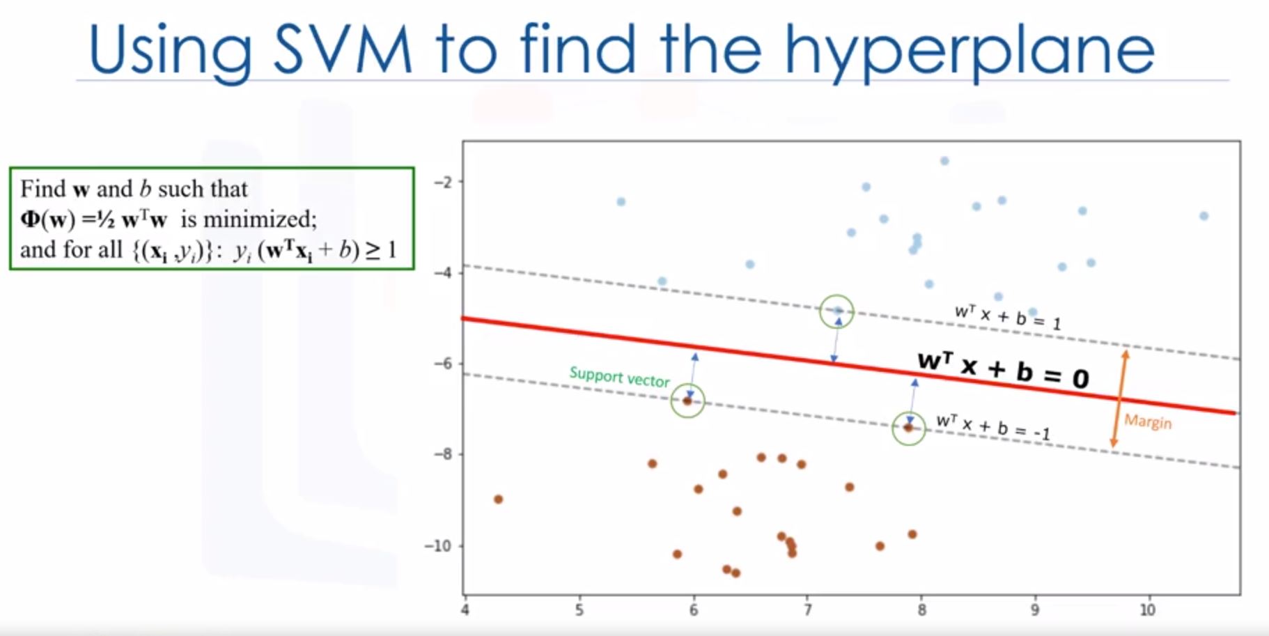
  • 2nd question: how can we find the best or optimized hyperplane after transformation? -> Using SVM
• Data transformation: maping data into a higher-dimensional space is called kernelling -> math function used is called kernel (linear, polynomial, Radial basis function - RBF, Sigmoid)
  • We usually choose different functions in turn and compare the results.
• One reasonable choice as the best hyperplane is the one that represents the largest separation or margin between the two classes.
  • Examples closest to hyperplane are support vectors.
  • Minimize the margin -> optimize parameters -> can use gradient descent!
• Pros and cons of SVM
  • Advantages: accurate in high-dimensional spaces + memory effecient
  • Disadvantages:
    • Prone to overfitting: if number of features are larger than number of samples.
    • Don’t provide probability estimation
    • Not efficient if your data is very big!
• Application of SVM
  • Image / hand written digit recognition
  • Text category assignment
  • Detecting spam
  • Gene Expression classification
  • Sentiment analysis
  • Regression, outlier detection and clustering

The lab of SVM

Link to ref.

Take a look on different class in scatter plots

ax = cell_df[cell_df['Class'] == 4][0:50].plot(kind='scatter', x='Clump', y='UnifSize', color='DarkBlue', label='malignant');
cell_df[cell_df['Class'] == 2][0:50].plot(kind='scatter', x='Clump', y='UnifSize', color='Yellow', label='benign', ax=ax);
plt.show()

Look at columns data types

cell_df.dtypes

Change to np arrays

feature_df = cell_df[['Clump', 'UnifSize', 'UnifShape', 'MargAdh', 'SingEpiSize', 'BareNuc', 'BlandChrom', 'NormNucl', 'Mit']]
X = np.asarray(feature_df)

cell_df['Class'] = cell_df['Class'].astype('int') # change to numeric, only 2 values 2 and 4
y = np.asarray(cell_df['Class'])

Train/test split

X_train, X_test, y_train, y_test = train_test_split( X, y, test_size=0.2, random_state=4)

Using SVM with kernel RBF (radial basis function)

from sklearn import svm
clf = svm.SVC(kernel='rbf')
clf.fit(X_train, y_train)
yhat = clf.predict(X_test)

Evaluation

from sklearn.metrics import classification_report, confusion_matrix

# f_1 score
from sklearn.metrics import f1_score
f1_score(y_test, yhat, average='weighted')

# jaccard index
from sklearn.metrics import jaccard_similarity_score
jaccard_similarity_score(y_test, yhat)