
IBM Data Course 6: Data Analysis with Python
Posted on 13/04/2019, in Data Science, Python.This note was first taken when I learnt the IBM Data Professional Certificate course on Coursera.
settings_backup_restore
Go back to Course 5: Week 3 & 4.
keyboard_arrow_right
Go to Course 7.
tocIn this post
Week 1: Importing Datasets
- Why Data Analysis
- Data is everywhere: collected by Data Scientist or automatically (when you click somewhere on the website, for example)
- Data is not information, with Data analysis/data science, it’s information
- Data Analysis plays an important role in
- Discovering useful info
- Answering questions
- Predicting future or the unknown
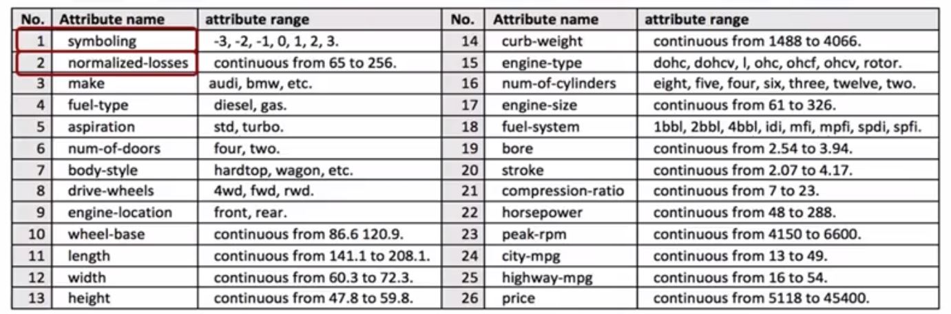
- Example (example csv file here)
- CSV = comma-separated values.
- Tom want to sell a car but which price is reasonable?
- Is there data on the prices of other cars and their characteristics?
- What features of cars affect their prices? (color, brand, horsepower, else?)
- We need data and how to understand data
- Understanding data
- Using CSV
- Each line represents a row
- Each of the attributes in the dataset
- Using CSV
- Python Packages for DS
- We have divided the Python data analysis libraries into three groups.
- Scientifics computing libraries:
- Pandas (data structures & tools): primary instrument -> data frame (2 dimensional table)
- Numpy (arrays & matrices)
- Scipy (integrals, solving differential equatins, optimization)
- Visualization Libearies
- Matplotlib (plots & graphs, most popular)
- Seaborn (based on matplotlib, plots: heat maps, time series, violin plots)
- Algorithmic libraries: machine learning -> develop a model using data + obtain predictions
- Scikit-learn (machine learning: regression, classification,clustering…): built on Numpy, Scipy and Matplotlib
- Statsmodels (Explore data, estimate statistical models and perform statistical tests)
- Scientifics computing libraries:
- We have divided the Python data analysis libraries into three groups.
- Importing and Exporting Data in Python:
- Process of loading and reading data into Python from various resources.
- Two important properties
- Format: the way data is encoded. Various format (.csv, .json, .xlsx, .hdf,…)
- Path: where data is stored (local or online)
- In python:
pd.read_csv(),pd.read_json(),pd.read_excel(),pd.read_sql()and the same forpd.to_??()import pandas as pd url = "path/to/data/file/" df = pd.read_csv(url) df.to_csv(path) // export to another csv file // without header df = pf.read_csv(url, header=None) // print nth first/last rows df.head(n) df.tail(n) - Replace default header
  headers = ["col1", "col2", "col3"]
  df.columns = headers
- Getting Started Analyzing Data in Python:
- Understand your data before you begin any analysis
- Pandas type: object, int64, float64, datetime64, timedelta[ns] (different from native python types)
- Check the data types of objects:
pd.dtypes - Return the statistical summary:
df.describe()- Full summary:
df.describe(include = 'all') - Or:
df.info()
- Full summary:
Week 2: Data Wrangling
- Pre-processing Data in Python
- Mapping raw form to another format to prepare for further analysis.
- Other calls: data cleaning / data wrangling
- Task:
- Identify + handle missing values
- Data formatting
- Data normalization (centering/scaling)
- Data Binning: creates bigger categories from a set of numerical values. It is particularly useful for comparison between groups of data.
- Turning categorical values to numeric variables
- Dealing with missing values
- They could be presented as:
?,N/A, - Drop the missing values: drop the variable, drop the data entry (if you don’t have many observation):
df.dropna() df.dropna(axis=0) // drop entire row df.dropna(axis=1) // drop entire column // drop some row whose missing value in colum 'price' df.dropna(subset=["price"], axis=0, inline=True) // inline means df will be modified after this method is applied df.dropna(subset=["price"], axis=0) // doesn't change df -> good way to be sure you're performing the correct the copperation - Replacing missing values:
- replace it with an avarage
- replace it by frequency (values appear most often)
- replace it based on other functions
  df.replace(<missing value>, <new value>)

  mean = df["col1"].mean()
  df["col1"].replace(np.nan, mean)
- Leaving it as missing value
- They could be presented as:
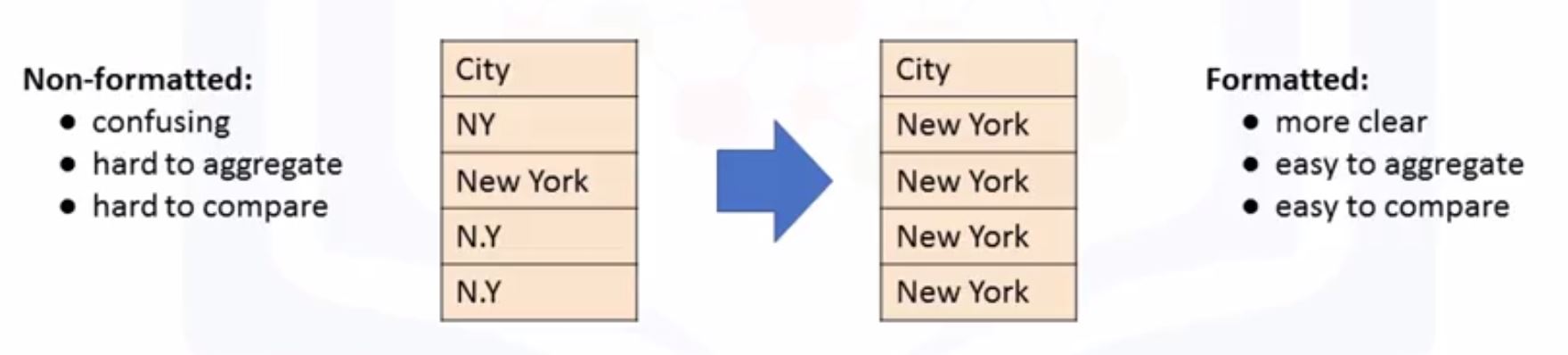
- Data Formatting in Python
- Change mile per galon (mpg) to litre per km (l/100km):
df["col1"] = 235/df["col1"] - Rename a column:
df.rename(columns={"col_old": "col_new"}, inplace=True) - Somtimes, incorrect data types.
- objects: “a”, “hello”,…
- int64: 1,3,5
- float: 1.2
- others
- Check data type:
df.dtypes() - Convert data type:
df.astype(), e.g.df["price"].astype("int")
- Change mile per galon (mpg) to litre per km (l/100km):
- Data Normalization in Python
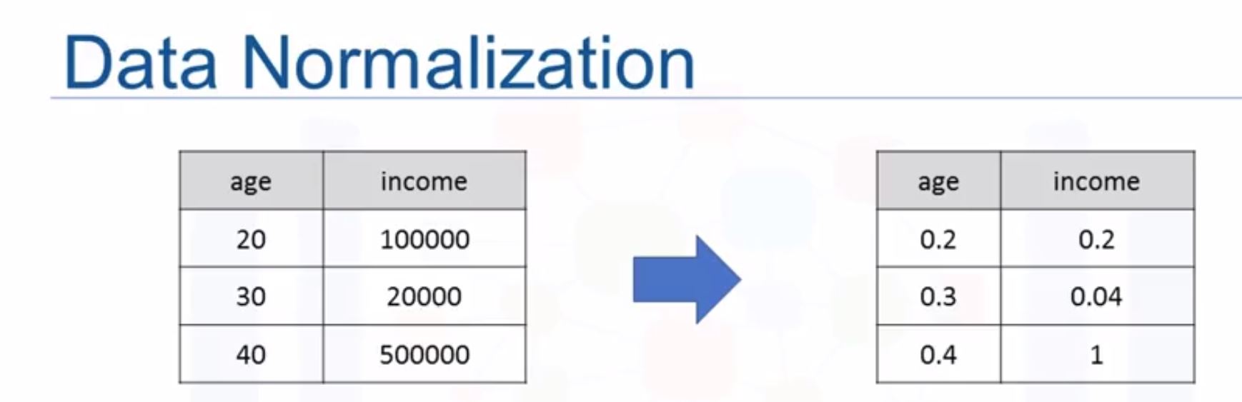
- diff ranges, hard to compare, the bigger will influnce the result most.
- Diff approaches
- Simple feature scaling: $x_{new} = \dfrac{x_{old}}{x_{max}}$
- Min-max: $x_{new} = \dfrac{x_{old}-x_{min}}{x_{max}-x_{min}}$
- Z-score: $x_{new} = \dfrac{x_{old}-\mu}{\delta}$, usually between (-3,3) based on normal distribution.
  df["col1"] = df["col1"]/df["col1"].max() // simple feature scaling
  df["col1"] = (df["col1"] - df["col1"].min())/(df["col1"].max() - df["col1"].min()) // min-max
  df["col1"] = (df["col1"] - df["col1"].mean())/df["col1"].std()
- Binning
- “Groups of values into bins”

bins = np.linspace(min(df["price"]), max(df["price"], 4)) // make 4 equal spaced numbers group_names = ["low", "medium", "high"] df["price-binned"] = pd.cut(df["price"], bins, labels=group_names, inlcude_lowest=True) - “Groups of values into bins”
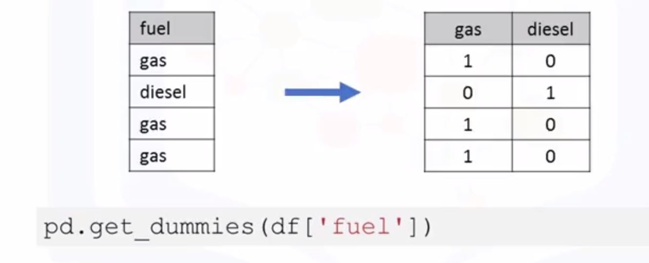
- Turning categorical variables into quantitative variables in Python
- Problem: most statistical models cannot take in the objects/strings as input
- Solution: assign 0 or 1 in each category -> One-hot encoding
Week 3: Exploratory Data Analysis
- Exploratory Data Analysis (EDA):
- Summary main characteristics of data
- Get better understanding about data
- Uncover relations between variables
- Extract import variables
- Descriptive Statistics
df.describe(): NaN will be excluded- Summerize the categorical data is by using
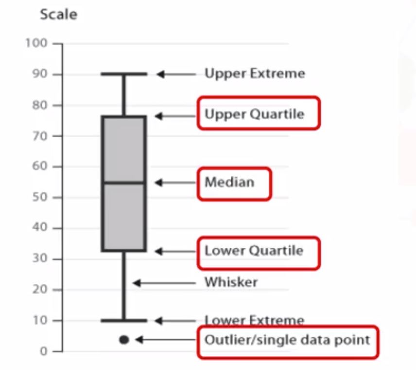
df.value_counts() - Using box-plots (Seaborn package)
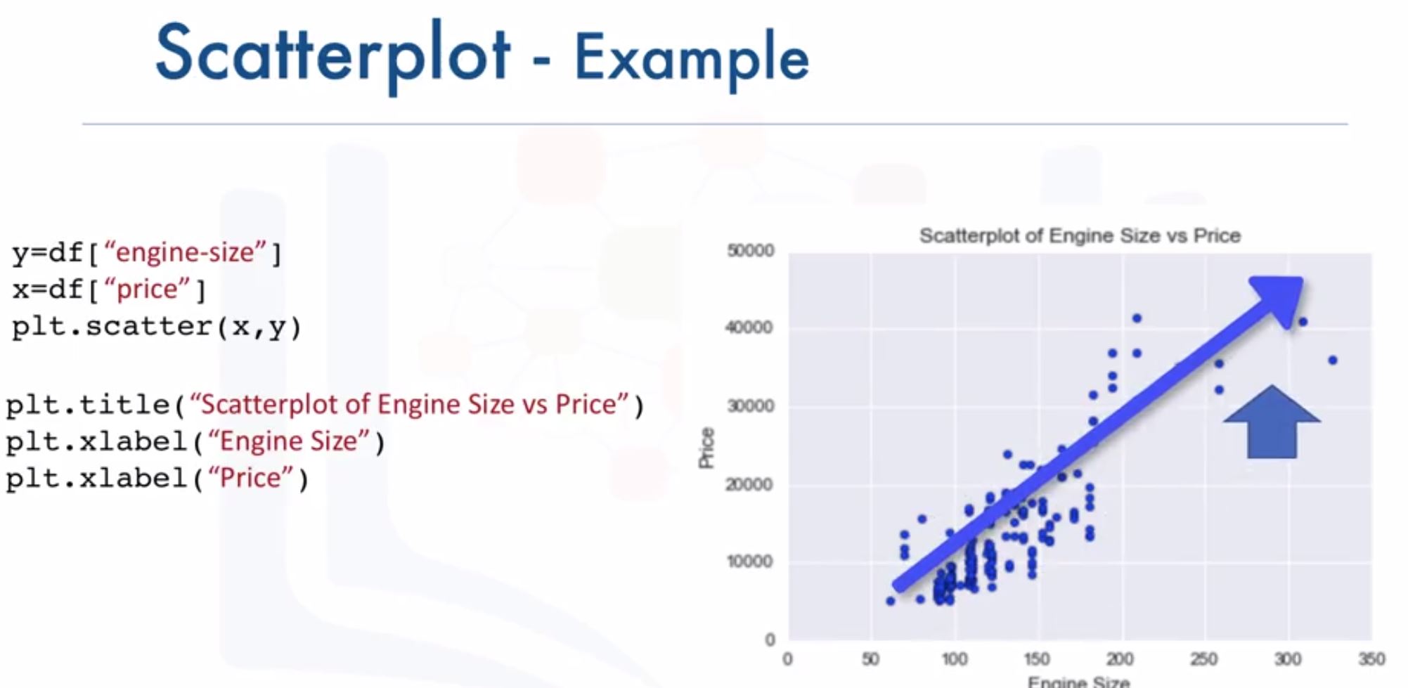
- Scatter plot: relationship between 2 variables
- GroupBy in Python
- group data into categories
- find the average “price” of each car based on “body-style”
df[['price','body-style']].groupby(['body-style'],as_index= False).mean() df.pivot()makes table like excel, easier for visualizing. A pivot table has one variable displayed along the columns and the other variable displayed along the rows.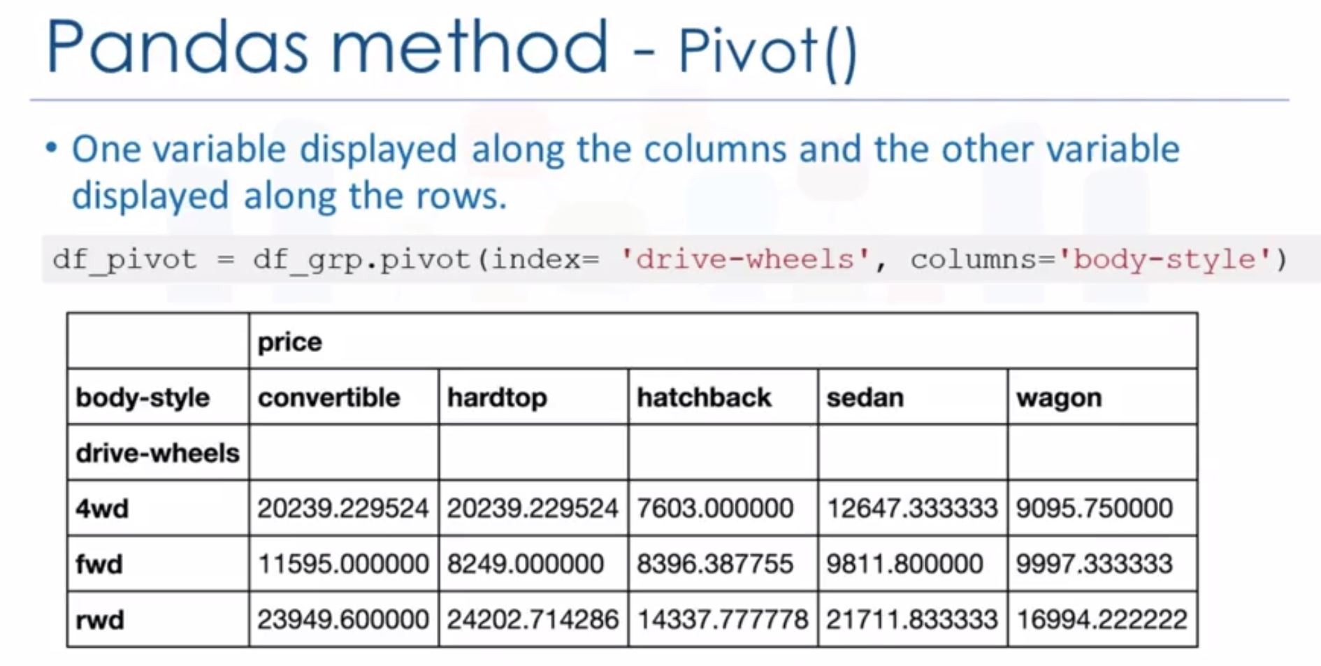
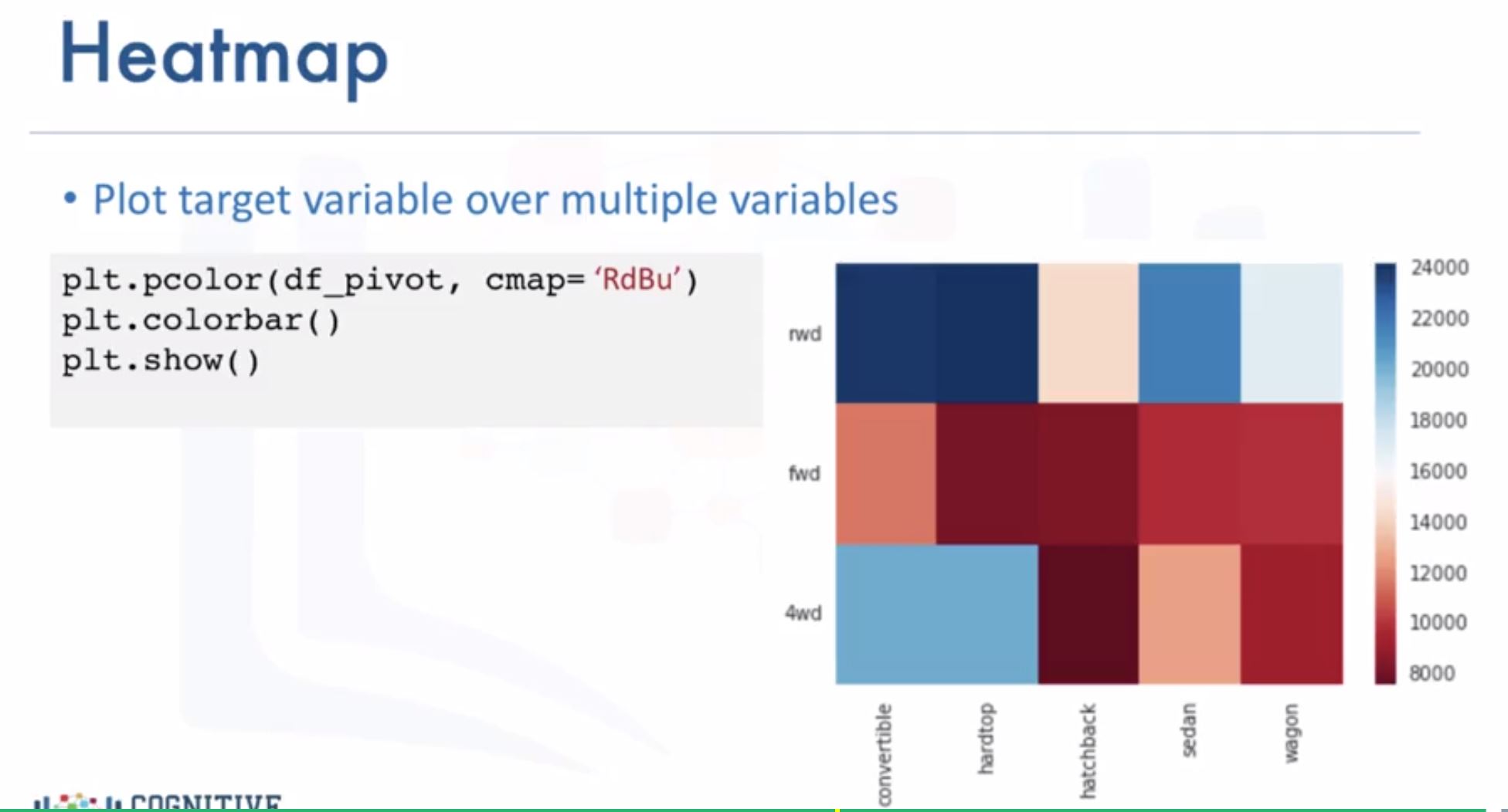
- Heatmap plot: plot the target variable over the multiple variable
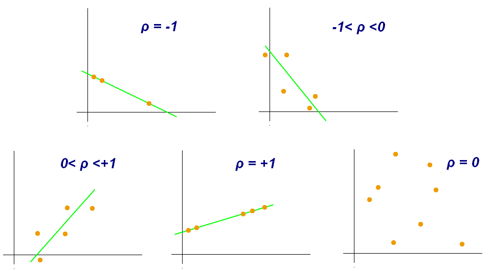
- Correlation
- Measure to what extent diff variables are interdependent
- Correlation doesn’t imply causation (quan hệ nhân quả): there a relation between A and B but we don’t have enough info to know which one causes the other?
- Correlation - Positive/negative Linear Relationship (y=ax, a>0 or a<0)
  sns.regplot(x="var1", y="var2", data=df)
  plt.ylim(0,)

  // or
  df[["col1", "col2"]].corr()
- Correslation - Statistics
- Pearson correlation: measures the strenght of correlation between 2 features
- Correlation coefficients
- p-value
- strong correlation: correlation close to 1 + p-value < 0.001
  import scipy.stats as stats
  pearson_coef, p_value = stats.pearsonr(df['col1'], df['col2'])
- Pearson correlation: measures the strenght of correlation between 2 features
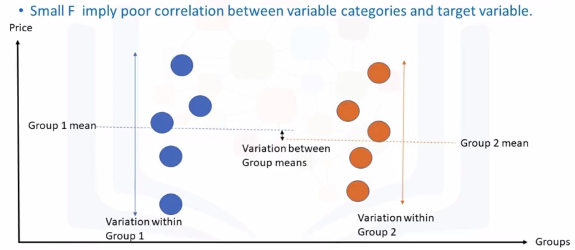
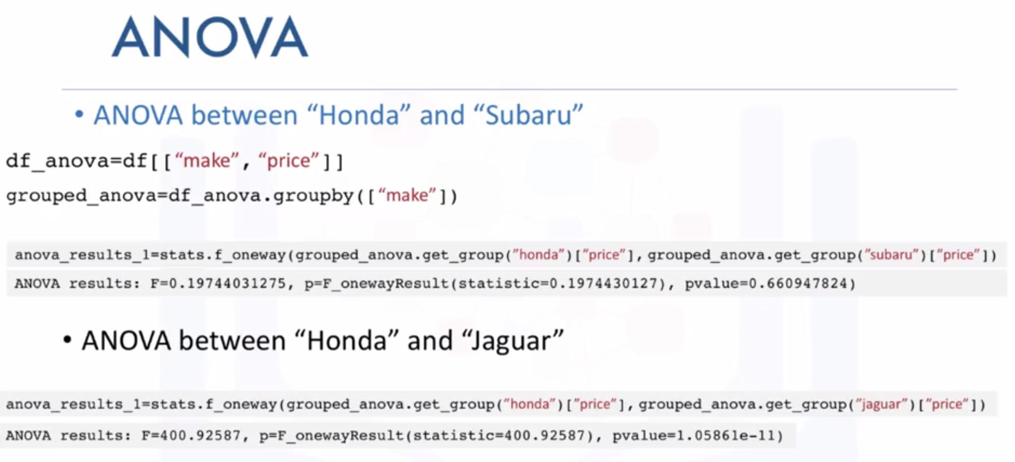
- Analysis of Variance (ANOVA)
- How impact of a categorical feature on the target?
- Finding correlation between diff groups of a categorical variable.
- What we obtain from ANOVA
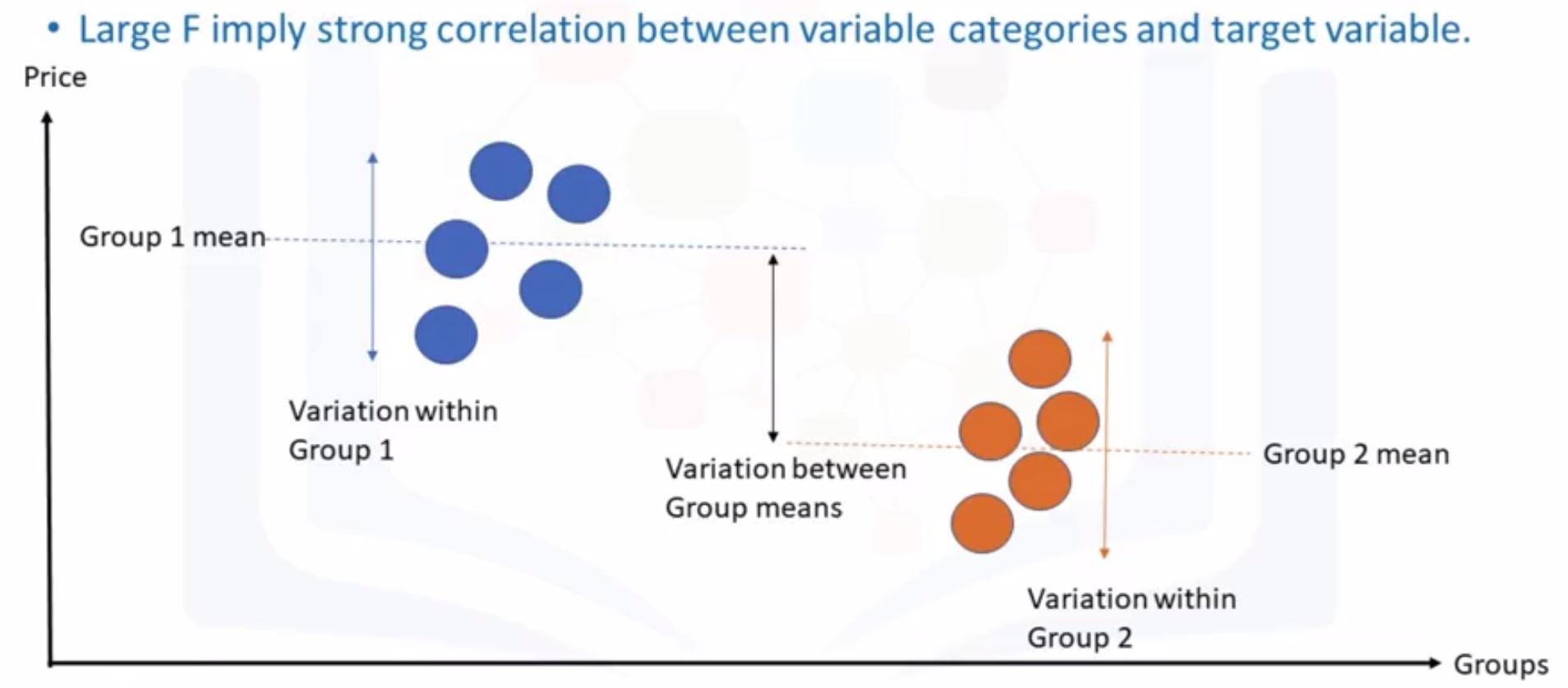
- F-test score: variation between sample group means divided by variation within sample group.
- p-value: confidence degree.
small F-score
big F-score
Week 4: Model Development
Check the lab for better understanding in a case-study.
- Model Development
- Linear Regression:
- the predictor (independent) variable x
- the target (dependent) variable y
- $y = b_0 + b_1x$ where
- $b_0$ is intercept:
lm.intercept_ - $b_1$ is slope:
lm.coef_
- $b_0$ is intercept:
// import from sklearn.linear_model import LinearRegression // create LR object lm = LinearRegression() // define variables X = df[["col1"]] Y = df[["col2"]] // fit lm.fit(X, Y) // predict Yhat = lm.predict(X) - Multiple Linear Regression
Z = df[["col1", "col2", "col3"]] Y = df[["coln"]] lm.fit(Z, Y) Yhat = lm.predict(X) - Model Evaluation using Visualization
- Regression plot
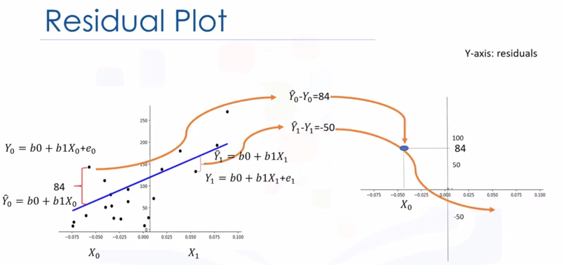
import seaborn as sns sns.regplot(x="col1", y="col2", data=df) plt.ylim(0,) - Residual plot: check diff actual values and predicted values
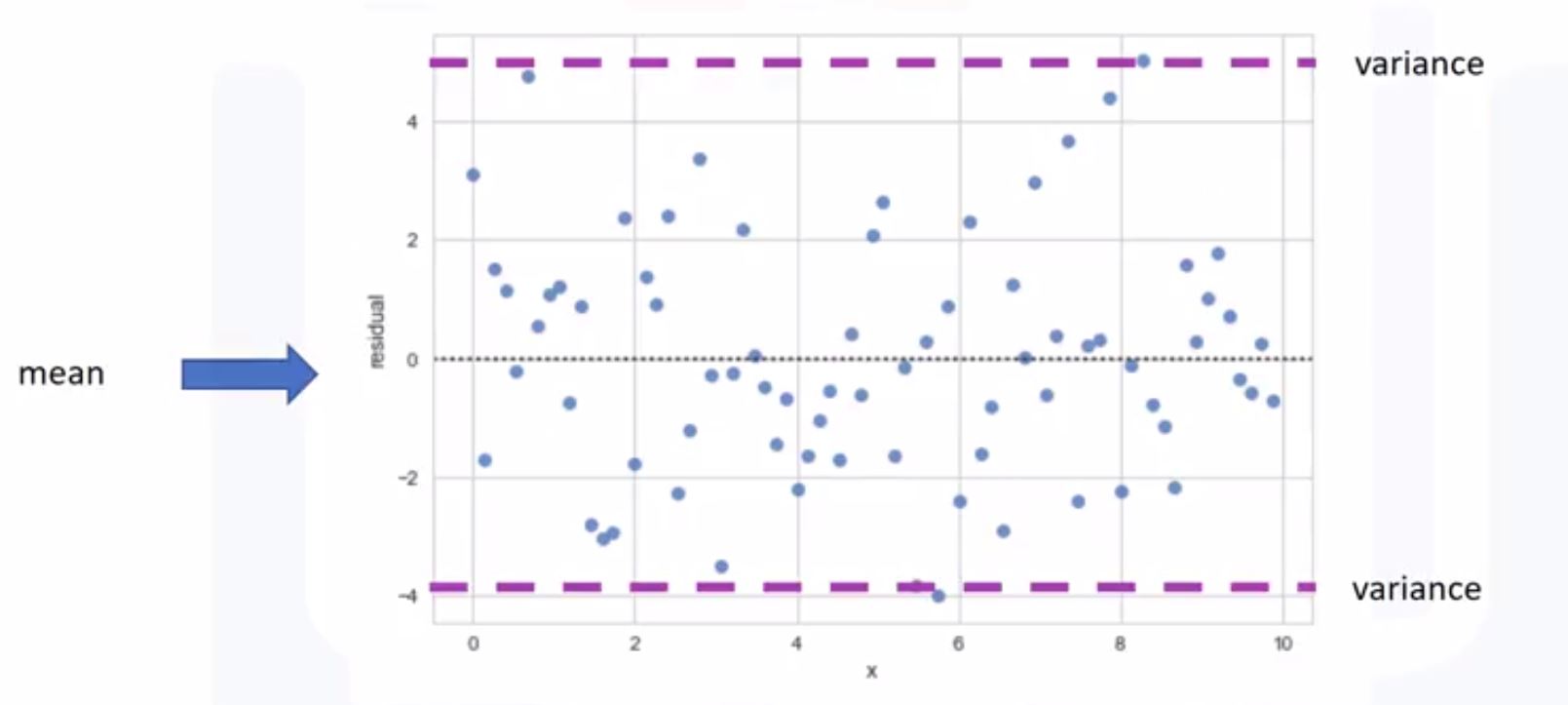
- If we have 0-mean, that’s linear regression
- Randomly spread out the x-axis
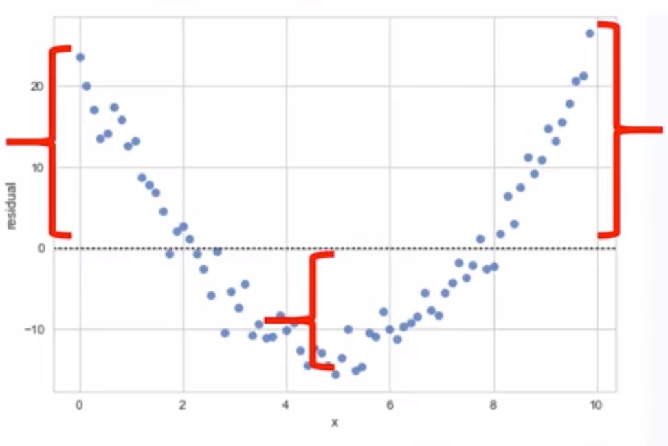
- If we don’t have 0-mean (sometimes positive, sometimes negative), that’s non-linear
- Not randomly spread out the x-axis.
Linear regression
Nonlinear
import seaborn as sns sns.residplot(df["feature"], df["target"]) - If we have 0-mean, that’s linear regression
- Distribution plot:
- counts predicted value versus the actual value
- These plots are extremely useful for visualizing models with more than one independent variable or feature.
- If we use multiple variables (left), the predicted is closed to actual
  import seaborn as sns
  ax1 = sns.distplot(df["price"], hist=False, color="r", label="Actual Value")
  sns.distplot(Yhat, hist=False, color="b", label="Fitted Value", ax=ax1)
- Regression plot
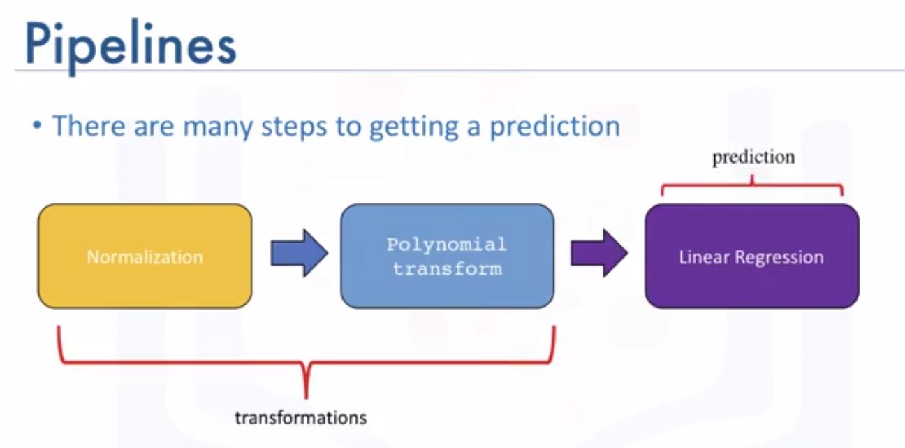
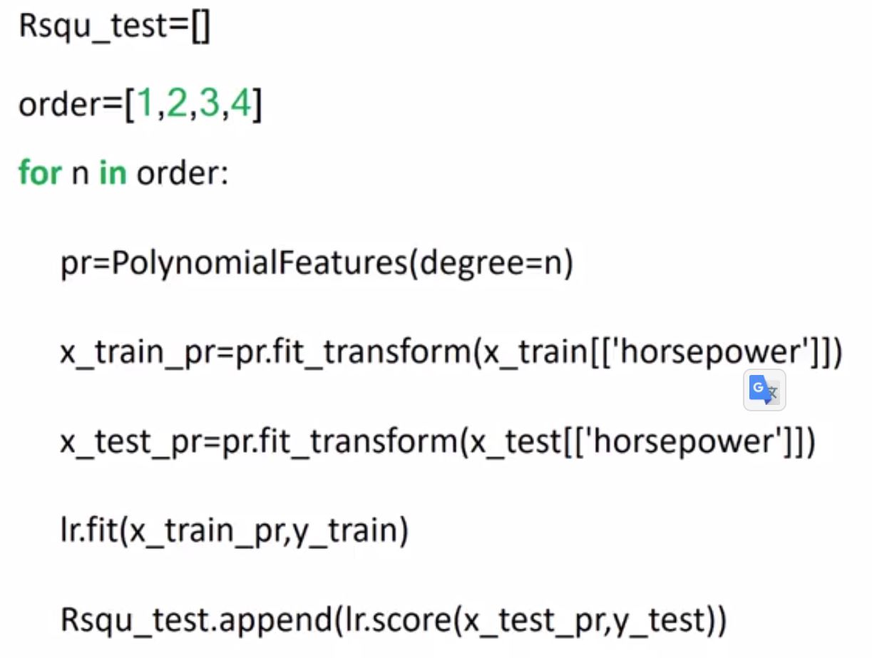
- Polynomial Regression and Pipelines
f = np.polyfit(x,y,3) // 3rd oreder polynomial p = np.poly1d(f) print(p) // print out the model : ax^3 + bx^2 + cx + d // polynomial with multiple variables from sklearn.preprogressing import PolynomialFeatures pr = PolynomialFeatures(degree=2, include_bias=False) x_polly = pr.fit_transform(x[["col1", "col2"]]) - We can normalize the each feature simultaneously
from sklearn.preprocessing import StandardScaler SCALE = StandardScaler() SCALE.fit(x_data[["col1", "col2"]]) x_scale = SCALE.transform(x_data[["col1", "col2"]]) - Pipelines: simplify the process of predicting (need to readmore about this!!!)
from sklearn.pipeline import Pipeline - Measures for In-Sample Evaluation
- Mean Square Error (MSE): difference between predicted values and actual values
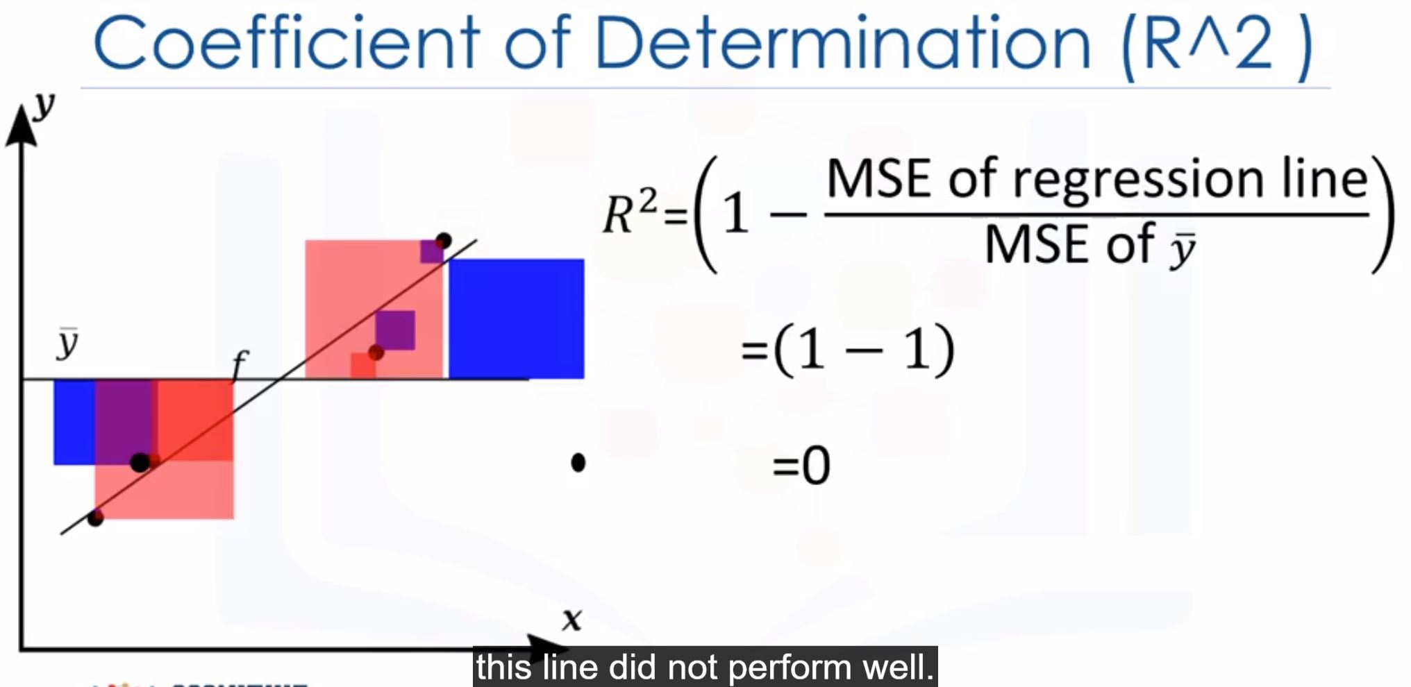
from sklearn.metrics import mean_squared_error mean_squared_error(df["col1"], Y_predict) - R-squared (Coefficient of Determination): how close the data is to the fited regression line
- Using:
lm.score(X, y) - Usually between 0 and 1
- If <0 -> overfitting
- Using:
- Mean Square Error (MSE): difference between predicted values and actual values
$R^2=1$ : good
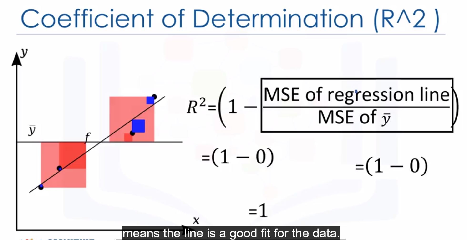
$R^2=0$ : worst
- Prediction and Decision Making
- See in the lab!!!
Week 5: Model Evaluation
Check the lab for better understanding in a case-study.
- Model Evaluation and Refinement: tells us how a model perform in the real world.
- In-sample evaluation tells us how well our model fits the data already given to train it.
- Problem: It does not give us an estimate of how well the train model can predict new data.
- Solution: in-sample (training data) and out-of-sample (test data)
- Split data set into: 70% training and 30% test:
from sklearn.model_selection import train_test_split - Generalization error is a measure of how well our data does at predicting previously unseen data.
- All our error estimates are relatively close together, but they are further away from the true generalization performance. To overcome this problem, we use cross-validation.
- It’s a model validation techniques for assessing how the results of a statistical analysis (model) will generalize to an independent data
- It is mainly used in settings where the goal is prediction, and one wants to estimate how accurately a predictive model will perform in practice.
- It is important the validation and the training set to be drawn from the same distribution otherwise it would make things worse.
- Why it’s helpful
- Validation help us evaluate the quality of the model
- Validation help us select the model which will perform best on unseen data
- Validation help us to avoid overfitting and underfitting.
  from sklearn.model_selection import cross_val_score

  sklearn.model_selection.train_test_split // make train/test
- In-sample evaluation tells us how well our model fits the data already given to train it.
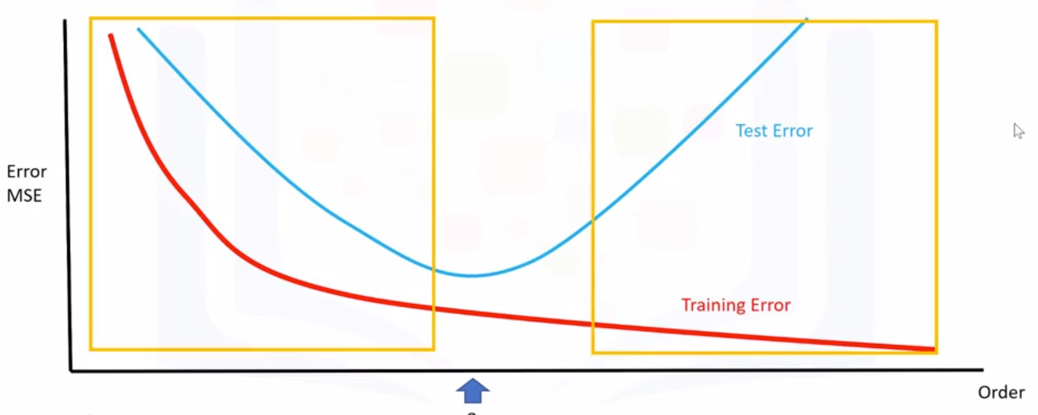
- Overfitting, Underfitting and Model Selection
- everything on the left box is considered as overfitting, right underfitting
- We can calculate different R-squared values as follows.
- everything on the left box is considered as overfitting, right underfitting
- Ridge Regression: prevent overfitting
- In polynomial equations, the coefficients going with the high order terms are very big. The Ridge regression will control these coefficients by introduce a parameter alpha.
- alpha too large -> these coeff seem to be zero -> underfitting
- alpha = 0 -> overfitting
- in order to track alpha, we use cross validation
- in Python
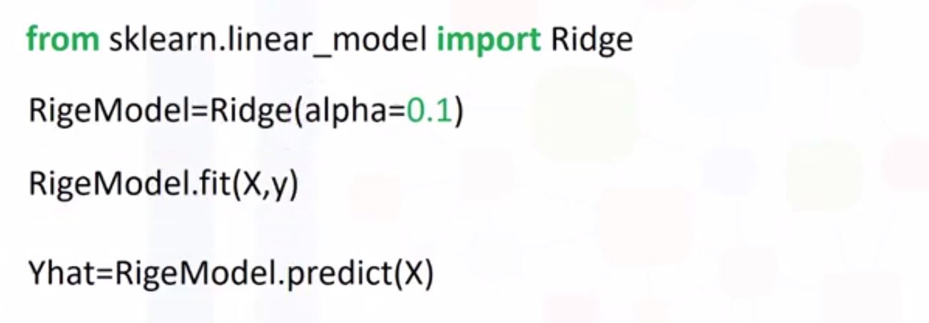
- To choose a good alpha, we start with the smaller one, increase step by step and then choose the one make R-squared values be max. Or with MSE.
- Minimize MSE or maximize R-squared.
- Grid Search
- Grid Search allows us to scan through multiple free parameters with few lines of code.
- Scikit-learn has a means of automatically iterating over these hyperparameters (like alpha) using cross-validation. This method is called Grid Search.
- What are the advantages of Grid Search is how quickly we can test multiple parameters.