
Stats 1
Posted on 11/08/2019, in Mathematics, Machine Learning, Data Science.Learn again Stats for Machine Learning and Data Science. A preparation step before writing articles on Math2IT.
References
- [1] Book: Understandable Statistics- Brase Brase BOOK.pdf
- Book: Think Stats 2 (with Python) - Allen B. Downey.
- Interactive book: Seeing Theory.
- probabilitycourse.com: an online book
- Stat Trek: teach yourself statistics.
Fundamental
General
-
face Khi nào thì PMF, CDF, PDF? Discrete vs Continuous? (ref)
Distribution Function
- The probability distribution function / probability function has ambiguous definition. They may be referred to:
- Probability density function (PDF) $\Rightarrow f_X(x)$
- Cumulative distribution function (CDF) $\Rightarrow F_X(x)$
- or probability mass function (PMF) $\Rightarrow p_X(x)$
- But what confirm is:
- Discrete case: Probability Mass Function (PMF)
- Continuous case: Probability Density Function (PDF)
- Both cases: Cumulative distribution function (CDF)
- Probability at certain $x$ value, $P(X = x)$ can be directly obtained in:
- PMF for discrete case
- PDF for continuous case
- Probability for values less than $x$, $P(X < x)$ or Probability for values within a range from $a$ to $b$, $P(a < X < b)$ can be directly obtained in:
- CDF for both discrete / continuous case
- Distribution function is referred to CDF or Cumulative Frequency Function (see this)
In terms of Acquisition and Plot Generation Method
- Collected data appear as discrete when:
- The measurement of a subject is naturally discrete type, such as numbers resulted from dice rolled, count of people.
- The measurement is digitized machine data, which has no intermediate values between quantized levels due to sampling process.
- In later case, when resolution higher, the measurement is closer to analog/continuous signal/variable.
- Way of generate a PMF from discrete data:
- Plot a histogram of the data for all the $x$’s, the $y$-axis is the frequency or quantity at every $x$.
- Scale the $y$-axis by dividing with total number of data collected (data size) $\Rightarrow$ and this is called PMF.
- Way of generate a PDF from discrete / continuous data:
- Find a continuous equation that models the collected data, let say normal distribution equation.
- Calculate the parameters required in the equation from the collected data. For example, parameters for normal distribution equation are mean and standard deviation. Calculate them from collected data.
- Based on the parameters, plot the equation with continuous $x$-value $\longrightarrow$ that is called PDF.
- How to generate a CDF:
- In discrete case, CDF accumulates the $y$ values in PMF at each discrete $x$ and less than $x$. Repeat this for every $x$. The final plot is a monotonically increasing until $1$ in the last $x$ $\longrightarrow$ this is called discrete CDF.
- In continuous case, integrate PDF over $x$; the result is a continuous CDF.
Why PMF, PDF and CDF?
- PMF is preferred when
- Probability at every $x$ value is interest of study. This makes sense when studying a discrete data - such as we interest to probability of getting certain number from a dice roll.
- PDF is preferred when
- We wish to model a collected data with a continuous function, by using few parameters such as mean to speculate the population distribution.
- CDF is preferred when
- Cumulative probability in a range is point of interest.
- Especially in the case of continuous data, CDF much makes sense than PDF - e.g., probability of students’ height less than $170$ cm (CDF) is much informative than the probability at exact $170$ cm (PDF).
- The probability distribution function / probability function has ambiguous definition. They may be referred to:
Random Variable (RV)
- Check this for a simple explanation and example.
- Discrete RV = a set of possible values from a random experiment.
- Continuous RV (ref $\Leftarrow$ good explanation!)
- If we want to define the probability of an event in which the random variable takes a specific value, the probability for this event will usually be zero $P(X=x)=0$ (vì khoảng là liên tục, chia ra $\infty$ khoảng nên là 0)
- Instead, we define the probability of events in which the random variable takes a value within a specific interval $\Rightarrow$ We can use CDF (Cumulative Distribution Function).
- [??] Ví dụ của continuous RV: (ref) the speed of car; The concentration of a chemical in a water sample; Measurement Errors; Electricity consumption in kilowatt hours.
- The set of possible values is called the Sample Space.
- A Random Variable has a whole set of values … and it could take on any of those values, randomly.
- Ex: X = {0, 1, 2, 3} and X could be 0, 1, 2, or 3 randomly.
- Probability: P(X = value) = probability of that value
[??] Nếu $X$ là 1 RV, vậy $X^2$ có thể được hiểu thế nào? Lấy ví dụ? / Multiplication of two random variable?. Nếu $X$ là “Số điểm trên mặt sau khi tung một con súc sắc.” thì $2X = X+X$ là gì và $X^2$ là gì?
$\Rightarrow$ $X+X$ chính là tổng điểm trên mặt của 2 lần tung. Còn $X^2$ chính là tích điểm trên mặt của 2 lần tung. Ví dụ, $X=1$ (1 lần tung được 1 nút), còn $Z=2X=5$ (2 lần tung được 5 nút) và $Z=X^2=4$ (2 lần tung được 4 nút). Tuy nhiên probability distribution sẽ thay đổi với $2X$ và $X^2$.
-
face Nói thêm!
- Convolution (tính chập, cf. def + ex): suppose $Z=X+Y$ and $X=x$ then the event $Z=z$ is equivalent to union of $(X=x)$ and $(Y=z-x)$. $\Rightarrow$ Có công thức tính theo $f_X$.
Xét $P(X=1)=\frac{1}{6}$ thì khi đó $Z=3X=X+X+X$ thì $P(Z=3)=?$. Có phải là
X=1 and X=1 and X=1?
Cón nếu Z=5 và Z=2X=X+X?
(X=1 and X=4) or (X=2 and X=2)?
P(and) = nhân, P(or) = cộng!
Ta có thể chuyển câu hỏi về what is the distribution of Z?: As a simple example consider X and Y to have a uniform distribution on the interval (0, 1). The distribution of their sum is triangular on (0, 2). (ref)
 Check the proof.
Mean - Median - Mode
- Có sự khác biệt giữa rời rạc và liên tục (continuous probability distribution).
- Nếu rời rạc thì dễ hiểu rồi.
- Nếu liên tục:
- Mean: Cái giúp cân bằng nếu để trên 1 cái tam giác.
- Median: Cái chia đôi diện tích.
- Mode: Cái cao nhất!
Probability mass function (PMF)
- Good explanation.
-
The probability distribution of a discrete random variable is called the probability function or the probability mass function (aka PMF). $\Rightarrow$ chỉ có cho discrete, còn liên tục thì $P(X=x)=0$.
- Properties:
- $0\le p_X(x) \le 1$.
- $\Sigma_x p_X(x)=1$.
Cumulative distribution function (CDF)
- The CDF of a real-valued random variable X, or just distribution function of X, evaluated at x, is the probability that X will take a value less than or equal to x.
- Cummylative = lũy tích -> tích lũy xác suất cho đến $x$.
- Discrete ($\Sigma$), continuous ($\int$).
$$ \begin{align} F_X(x) &= P(X\le x) = (\Sigma_{t\le x}f(t)) = (\int_{-\infty}^xf_X(t)dt). \\ P(a<X\le b) &= F_X(b) - F_X(a). \\ \bar{F}_X(x) &= P(X>x) = 1-F_X(x). \end{align} $$ - Properties:
- $0 \le F_X(x) \le 1$
- CDF a non-decreasing function, or monotonically increasing because we are adding up the probabilities for each outcome.
- CDF is said to be a continuous function, (it has no “holes” in the graph)
- $\lim_{x\to -\infty}F_X(x)=0$, $\lim_{x\to +\infty}F_X(x)=1$
- [??] - Tại sao $a<X$ mà không phải là $a\le X$? $\Rightarrow$ tại vì nó đã bị trừ trong cái $-F_X(a)$.
- Dấu "=" chỉ quan trọng với discrete variable, continuous variable không quan trọng lắm!
Probability density function (PDF)
- PDF or density of a continuous random variable: $f_X(x)$
- The PDF is used to specify the probability of the random variable falling within a particular range of values
- Its value at any given point is actually meaningless: trên khoảng thì có xác suất là $\int$ trên khoảng đó nhưng tại 1 điểm thì ko có xác suất (nếu xét theo ý tưởng chia cho $\infty$ miền nhỏ)! Tuy nhiên, ta vẫn có thể tính xác suất của 1 biến continuous X tại 1 điểm:
- The PDF is the density of probability rather than the probability mass
- Properties:
- $f_X(x) = F’_X(x)$
- $f(x)\ge 0, \forall x$
- $\int_{-\infty}^{\infty}f(x) dx =1$
- $P(a\le X\le b)= \int_a^bf(x)dx, \forall a,b$ (probabilities = area under the curve $f(x)$)
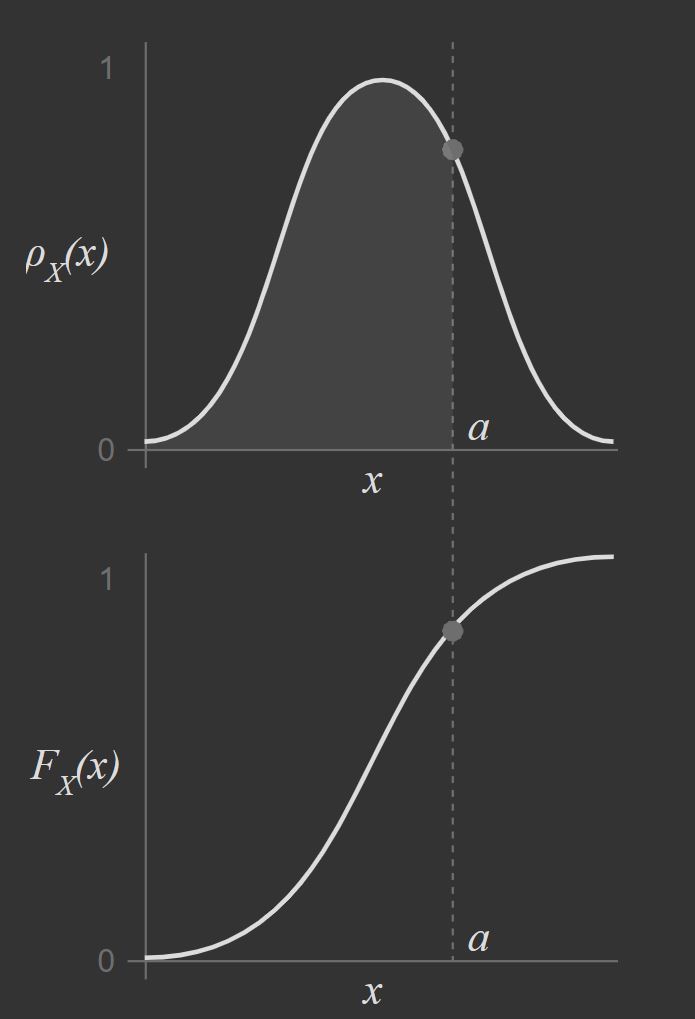
- [??] Relationship between a PDF (hình trên) and the CDF (hình dưới). Ref.
- CDF $\Rightarrow$ trên graph chỉ là tại 1 điểm nhưng giá trị thật ra là trên 1 khoảng (trên PMF hoặc PDF)
- PDF $\Rightarrow$ diện tích của 1 dãy tới điểm đang xét / tổng diện tích!
- Other ideas/explanation: [mathinsight]
Expected value
Có thể tham khảo interactive prob tại đây.
Expected value = Mean = (intuitively) the long-run average of occurrences.
- Discrete: $\mu = E(X) = \Sigma[xP(x)]$
- Continuous: $\mu=E(X) = \int_{\mathbb{R}} xf_X(x) dx$ where $f_X$ is PDF (probability density function)
[??]: Hiểu công thức của Continuous như thế nào? (Discrete thì dễ rồi, nó là weight*value thôi).
- Trước hết phải hiểu PDF là gì? (Xem bên dưới)
- Sau khi hiểu $f_X$ rồi thì $f_X(x)$ cũng là xác suất của $X$ tại $x$ (Tượng trưng là $P(X=x)$ nhưng P này =0 trong trường hợp X continuous này!).
Expectation of Function of Discrete Random Variable (ref + proof):
Variance
Variance = Whereas expectation provides a measure of centrality, the variance of a random variable quantifies the spread of that random variable’s distribution.
- Tưởng tượng nó giống trung bình khoảng cách khác biệt giữa $\bar{y}$ và $y$.
[??] Hiểu hai dấu bằng trên như thế nào? $\Leftarrow$ Thật ra nên hiểu trực quan về Variance như ở dưới hơn là hiểu về 2 dấu bằng này! $\Rightarrow$ Xem ở đây
- Dấu bằng thứ 1: ta sẽ xem xét sự khác biệt giữa X và giá trị trung bình (mong muốn) của nó xem sao. Tuy nhiên, có nhiều cái X khác nhau (thử tưởng tượng trường hợp rời rạc), nên ta phải lấy trung bình của nó.
- Dấu bằng thứ 2: Liệu sau khi $X^2$ thì trung bình của nó có giống với trước khi nó bình phương hay không?
[??] Vẫn chưa hiểu mối liên quan (trực quan) giữa 2 dấu bằng là sao? (về mặt toán học thì có thể chứng minh được nhưng về mặt ý nghĩa trực quan thì giải thích làm sao?)
Hiểu trực quan: variance ($\sigma^2$) và standard deviation ($\sigma$) cho chúng ta biết mức độ phân tán của dữ liệu so với mean của chúng. Nếu variance lớn tức mức độ phân tán cao (nhìn vào graph của normal distribution để hiểu thêm).
Distributions
What’s a distribution?
[??] Why a random variable has a probability distribution? $\Rightarrow$ Mỗi RV có thể nhận bất kỳ giá trị nào trong sample space của nó (Ví dụ tung 2 súc sắc thì khả năng cao sẽ được 7 nút hơn là được 12 nút, do expected value sẽ là 3.5 cho mỗi con ss). Do đó, mỗi CV cũng sẽ có 1 probability distribution riêng ám chỉ có bao nhiêu khả năng mà X đó sẽ nhận giá trị x trong cái sample range kia (ref more).
[??] How to find feature distribution in Python?
DataFrame.hist(bins=10)
#Make a histogram of the DataFrame and then check
Uniform Distribution (continuous)
- Also called Rectangular Distribution (ref)
- It has equal probability for all values of the Random variable between a and b.
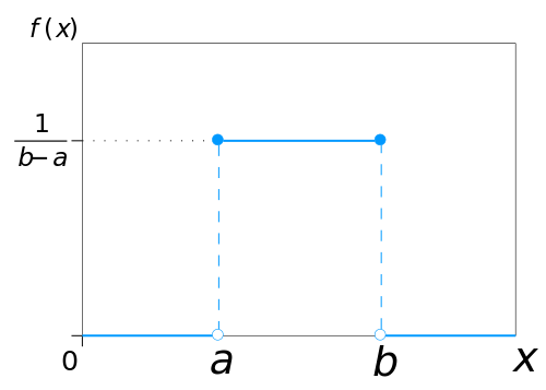 Probability density function
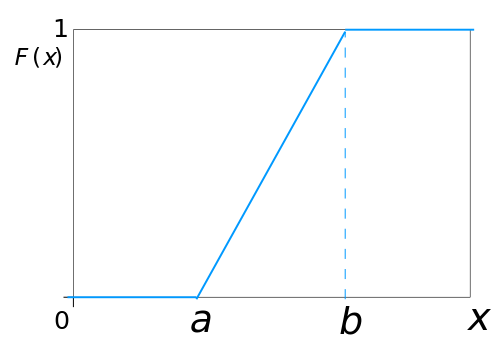 Cumulative distribution function
- Mean = Median = $\frac{a+b}{2}$.
- Mode = any values in (a,b).
- Variance = $\frac{(b-a)^2}{12}$
Normal distribution (continuous)
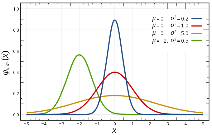 Probability density function
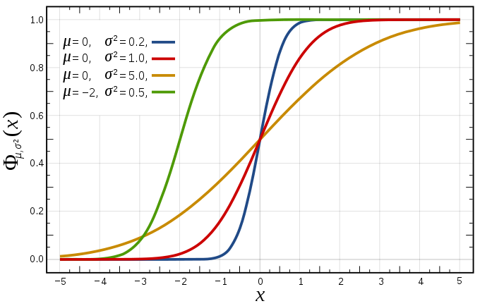 Cumulative distribution function
- Mean = Median = Mode = $\mu$.
- Variance = $\sigma^2$.
- Informally called bell curve (tuy nhiên còn nhiều distribution khác cũng có bell shape!)
- Bài viết hay: mathisfun
- Bài viết chi tiết khác: file (đã backup ở the_normal_distribution_notes.pdf)
- Đặc trưng: mean ($\mu$) and standard deviation ($\sigma$) (Deviation means “distance from the mean”.)
- Nếu một biến ngẫu nhiên X có phân phối chuẩn thì: $X\sim \mathcal{N}(\mu, \sigma)$.
- Ví dụ của “not a normal distribution”: xúc xắc, điểm thi của học sinh lớp 9 khi làm đề lớp 8.
- Trò Quincunx cho 1 ví dụ của cái normal dist này (các viên bi rơi ngẫu nhiên xuống 1 tam giác có nhiều chướng ngại)
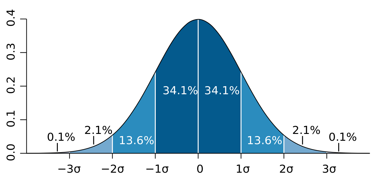
- 68-95-99.7 rule (**Empirical rule**)
- 68% ($\mu-\sigma, \mu+\sigma$), 95% ($\mu-2\sigma, \mu+2\sigma$), 99.7% ($\mu-3\sigma, \mu+3\sigma$)
- [??] Tại sao giữa $(0,\delta)$ thì là 34.1% nhưng giữa $(-\delta, \delta$) lại là 68%? $\Rightarrow$ Chỉ là xấp xỉ mà thôi (để có cái tên gọn gọn của 68-95-99.7 rule)
-
Standard normal distribution: when $\mu=0, \sigma=1$ or $X\sim \mathcal{N}(0,1)$.
 Cách standardize này dùng công thức tính z-score là được!
 - [??] Tại sao phải standardize? $\Rightarrow$ It can help us make decisions about our data.
- Giả dụ sau khi có kết quả thi, toàn điểm trên thang 100 nhưng khá thấp. Nếu chúng ta dựa vào đó thì không biết nên lấy điểm sàn là bao nhiêu. Tuy nhiên khi chuyển về standard normal dist (dựa trên điểm trung bình của đám sinh viên đã thi), ta có thể chọn được điểm sàn rõ ràng và công bằng hơn! (ref)
[??] Dấu hiệu nhận biết của normal distribution là gì? $\Leftarrow$ Thật ra không biết có dấu hiệu hay không, chỉ biết là nó rất phổ biến trong tự nhiên + khi ứng dụng Central Limit Theorem thì đều converge về nó!
- Nếu một biến ngẫu nhiên mà chưa được biết distribution gì thì ta thường dùng cái ND này!
- Nhờ vào Central Limit Theorem, càng nhiều observations thì có khả năng cao X càng converge về ND.
import numpy as np

# raw random samples from a normal distribution
np.random.normal(loc=0, scale=1.0, size=None)

# loc = mean, scale = sd, (size)
# returns ndarray/scalar
- Plot/more examples on numpy.
Z-Scores (standard score)
- Liên quan đến Normal distribution!
- Khi ta muốn biết mình đứng thứ mấy trong lớp sau khi có điểm bài kiểm tra?
- One statistic that is used to measure the position of a data value w.r.t. other data values is known as the z-score.
-
z-score of a x = number of SD from the mean to that x.
$$ z_X = \dfrac{x-\mu}{\sigma}. $$ - z-score is dimensionless measure.
- z-score (>0) càng lớn thì x càng nằm trong top cao so với trung bình.
- z-score (<0) càng bé thì x càng nằm trong top thấp so với trung bình.
- EX: sau khi tính điểm trung bình của 2 đợt thi, lần 1 $z_x=0.375$, lần 2 $z_x=0.825$ thì ta sẽ biết được (nếu so với các bạn cùng lớp), lần 2 chúng ta làm bài tốt hơn nhiều!
Binomial distribution (discrete)
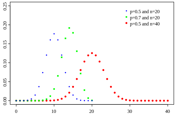 Probability mass function
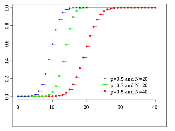 Cumulative distribution function
- When a RV has only 2 independent outcomes (giống như tung đồng xu). Each trial has the same probability.
- Usage: The binomial distribution is often used in social science statistics as a building block for models for dichotomous outcome variables, like whether a Republican or Democrat will win an upcoming election, whether an individual will die within a specified period of time, etc (ref).
- The binomial distribution determines the probability of observing a specified number of successful outcomes in a specified number of trials.
- Ex: Tung đồng xu 10 lần, 4 lần được mặt ngửa, biết xs được mặt ngử là 0.7: $n=10, k=4, p=0.7$ $\Rightarrow p_X = C_10^4 (0.7)^4 (0.3)^6$.
- [??] Hiểu PMF như thế nào?
- PMF: Giả sử ta xét n trials là 1 dãy hàng ngang n vị trí. Trong n trials ta chỉ được k trường hợp, mỗi trường hợp có xs đạt được là p nên đầu tiên ta cần chọn ra k vị trí thành công trước cái đã, có $C_n^k$ cách chọn vị trí này. Ứng với mỗi cách chọn k vị trí này, mỗi vị trí nếu muốn được thành công thì có xs là p nên k chỗ sẽ cần $p^k$. Đồng thời các chỗ còn lại phải không thành công (nếu không thì có thể có nhiều hơn k trường hợp thành công), do đó các chỗ ko thành công này nếu muốn đạt được thì ứng với $(1-p)^{n-k}$. Do tất cả các điều kiện này phải xảy ra dính líu đến nhau nên phải nhân chúng lại, hay ta được công thức của PMF.
- PDF: chỉ việc tổng hết các trường hợp lại thôi vì $X\le x$.
- Nếu một biến ngẫu nhiên X có phân phối binomial thì: $X\sim B(n,p)$.
- When $n=1$ then it’s Bernoulli distribution.
- Expected value (mean): $EX = n_{trials} \times p_{success}$
- Variance: $np(1-p)$ where $p$ is the proba of the success
- Median: there is no general result for this, but there is something interesting!
[??] Why we have E and EX like above?
- Expected: nếu ta tung đồng xu 100 lần, hẳn ta muốn thấy mặt ngửa 50% (= $n\times p$) số đó. Dễ hiểu!
- Variance: do X là n trial $X_i$ khác nhau, mỗi trial là 1 Bernoulli distribution nên ta chuyển việc hiểu variance về hiểu variance của Bernoulli distribution (ref).
Bernoulli distribution (discrete)
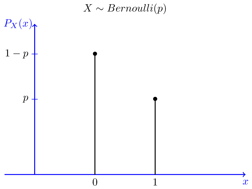 PMF of a Bernoulli random variable
- Xem wiki cho bảng tóm tắt mấy cái hàm.
- $X\sim B(1,p)$: special case of binomial distribution
- Tung đồng xu 1 lần duy nhất: xác suất để được mặt số 1 là p, mặt số 0 là 1-p, thế thôi.
- Mean: $EX = 1\times \Pr(X=1) + 0\times \Pr(X=0) = p$.
- Variance: check this, nhớ dùng Expectation of Function of Discrete Random Variable. Chỉ cần dùng công thức là ok.
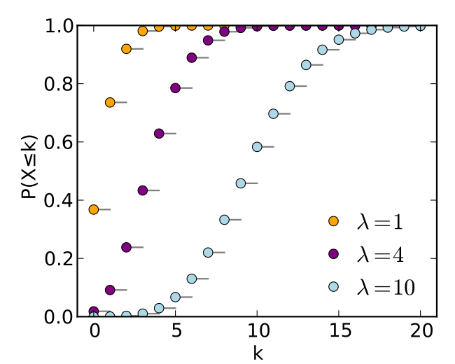
Poisson distribution (discrete)
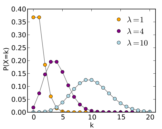 The horizontal axis is the index k, the number of occurrences. $\lambda$ is the expected number of occurrences, which need not be an integer. The vertical axis is the probability of k occurrences given $\lambda$. The function is defined only at integer values of k. The connecting lines are only guides for the eye.
 The horizontal axis is the index k, the number of occurrences. The CDF is discontinuous at the integers of k and flat everywhere else because a variable that is Poisson distributed takes on only integer values.
- $\lambda$ is the average number of events per interval
- $k$ takes values $0,1,2,\ldots$
- The poisson distribution is used to calculate the number of events that might occur in a continuous time interval.
- Examples:
- An individual keeping track of the amount of mail they receive each day may notice that they receive an average number of 4 letters per day. If receiving any particular piece of mail does not affect the arrival times of future pieces of mail, i.e., if pieces of mail from a wide range of sources arrive independently of one another, then a reasonable assumption is that the number of pieces of mail received in a day obeys a Poisson distribution.[ref]
- Other examples that may follow a Poisson distribution include the number of phone calls received by a call center per hour
- The number of decay events per second from a radioactive source.
Central Limit Theorem
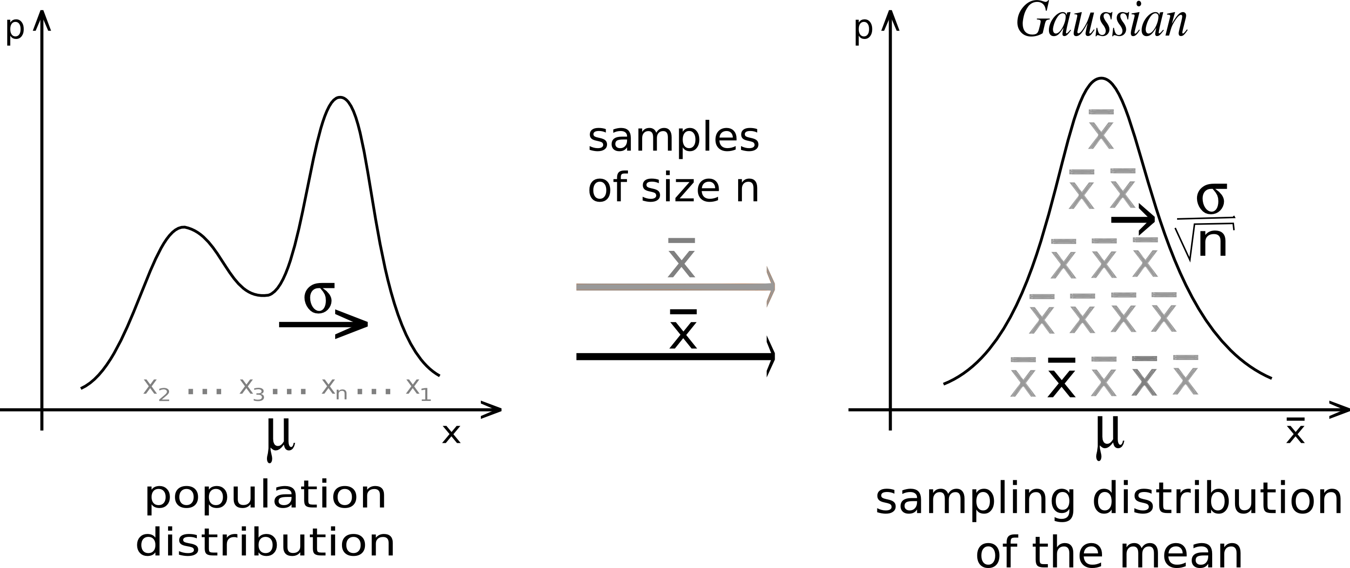 Whatever the form of the population distribution, the sampling distribution tends to a Gaussian, and its dispersion is given by the Central Limit Theorem.[ref]
- Định lý giới hạn trung tâm.
- The Central Limit Theorem for Any Probability Distribution: If x possesses any distribution with mean $\mu$ and standard deviation $\sigma$, then the sample mean $\bar{x}$ based on a random sample of size $n$ will have a distribution that approaches the distribution of a normal random variable with mean $\mu$ and standard deviation $\sigma/\sqrt{n}$ as $n$ increases without limit.
- But sample sizes are sometimes small, and often we do not know the standard deviation of the population. When either of these problems occur, statisticians rely on the distribution of the t statistic (also known as the t score).
[??] Ví dụ của một X không có normal distribution nhưng converge về ND?: [1] $\Leftarrow$ Thật ra dựa vào số lượng sample, ta có thể dự đoán mean và SD có thể convert về normal dist chứ thật ra một cái bất kỳ vẫn chưa tìm thấy ví dụ được!
[??] How large should the sample size be if we want to apply the central limit theorem? $\Rightarrow$ $n\ge 30$ nhưng đừng dùng nó mù quáng! (ref. Theorem 7.2 of book Understandable Statistics)
Using CLT ($\bar{x}$ distribution $\to$ normal distribution), we have:
where,
- $n$ is the sample size ($n\ge 30$)
- $\mu$ is the mean of $x$ distribution
- $\sigma$ is the SD of $x$ distribution.
t-values (Student’s t distributions, t-statistic, t-test)
- (ref - hay) The t distribution (aka, Student’s t-distribution) is a probability distribution that is used to estimate population parameters when the sample size is small and/or when the population variance is unknown.
- Student’s t distribution được khám phá bởi W.S. Gosset. Vốn dĩ nó có tên vậy là vì ngày đó cty ông đang làm cho không khuyến khích nhân viên của mình đăng báo riêng. Do đó ông đã lấy bút danh là Student. Ông đã dùng biến $t$ nên nó vẫn được giữ tên như vậy!
- Statistical methods for obtaining reliable information from samples of populations with unknown SD $\sigma$ (không biến độc phân tán dữ liệu ra sao!!!).
Student’s t distribution [1]
Assume that $x$ has normal distribution with mean $\mu$. For sample size $n$, with the sample mean $\bar{x}$ and sample standard deviation $s$, the t variable,
has a Student’s t distribution with degrees of freedom $n-1$.
-
There are actually many different t distributions. The particular form of the t distribution is determined by its degrees of freedom. The degrees of freedom refers to the number of independent observations in a set of data. (# of independent observations = dof-1)
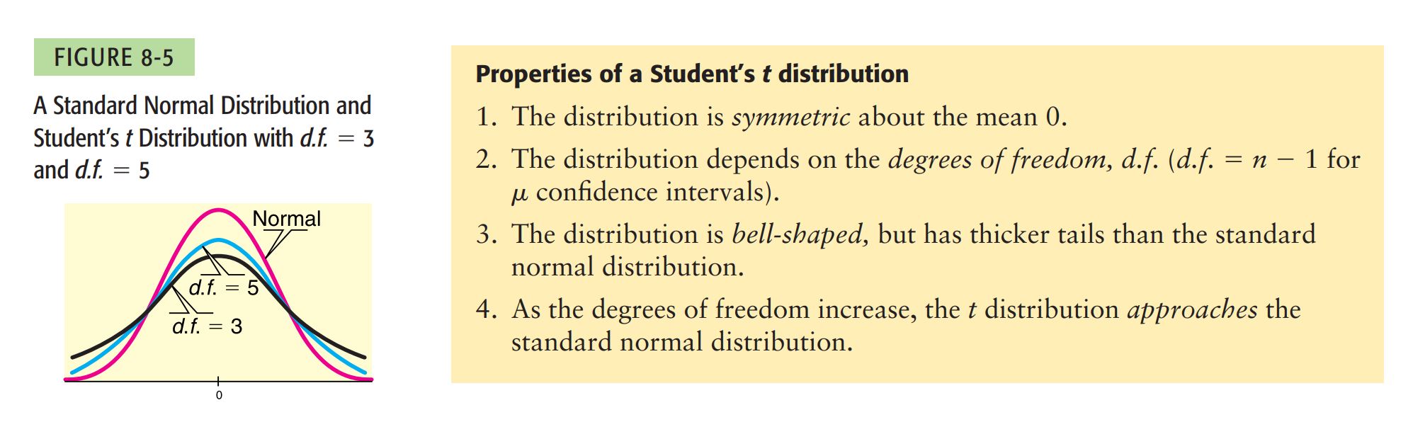
- # of dof càng lớn thì t-distributions càng gần normal distribution.
- The t distribution should not be used with small samples from populations that are not approximately normal.
- The t statistic produced by this transformation can be associated with a unique cumulative probability. [???]
-
face Examples
Problem: Acme Corporation manufactures light bulbs. The CEO claims that an average Acme light bulb lasts 300 days. A researcher randomly selects 15 bulbs for testing. The sampled bulbs last an average of 290 days, with a standard deviation of 50 days. If the CEO’s claim were true, what is the probability that 15 randomly selected bulbs would have an average life of no more than 290 days?
- Đầu tiên, tính t-statistics theo công thức ở trên: $t=- 0.7745966$
- dof = 15-1 = 14
- Sử dụng t-distribution calculator, nhưng ko biết nó tính thế nào????
Có thế nó tính theo $1-t$.
Xem thêm tại đây.
Confidence interval (CI) & uncertainly
- Refs: [1, p.345], [4]
- What is it?
- Confidence interval for mean $\mu$ when SD $\sigma$ is unknown: